Symmetry Autumn of Code 2020 Projects and Participants

Symmetry Investments logoThe verdict is in! Five programmers will be participating in the 2020 edition of the Symmetry Autumn of Code. Over the next three weeks, they will be working with their mentors to take the goals they outlined in their applications and turn them into concrete tasks across four milestones. Then, on September 15th, the first milestone gets under way.

Throughout the event, anyone can follow the progress of each project through the participants’ weekly updates in the General forum. Please don’t ignore those posts! You might be able to offer suggestions to help them along the way.

And now a little about the SAOC 2020 participants and their projects.

  • Robert Aron is a fourth-year Computer Science student at University POLITEHNICA of Bucharest. For his project, he’ll be implementing D client libraries for the Google APIs. When it’s complete, we’ll be able to interact with Google service APIs, such as GDrive, Calendar, Search, and GMail, directly from D. The goal is to complete the project by the end of the event.
  • Michael Boston is currently developing a game in D. For his SAOC project, he’ll be taking some custom data structures he’s developed and adapting them to be more generic. The ultimate goal is to get Michael’s modified implementation merged into Phobos. Should that not happen, the library will still be part of the D ecosystem once it’s complete.
  • Mihaela Chirea is a fourth-year Computer Engineering student at University POLITEHNICA of Bucharest. Mihaela will spend SAOC 2020 improving DMD as a library. Part of this project will involve soliciting community feedback regarding proposed changes, so anyone interested in using DMD as a library should keep an eye out for Mihaela’s posts in the D forums.
  • Teona Severin is a first-year master’s degree student at University POLITEHNICA of Bucharest who will be working on a mini DRuntime in order to bring D to low-performance microcontrollers based on ARM Cortex-M CPUs. Currently, D can run on such systems when compiled as -betterC, but the end goal of this project is to get enough of a functional DRuntime to write “a simple application that actively uses a class.“
  • Adela Vais is yet another fourth-year Computer Engineering student at University POLITEHNICA of Bucharest. For her project, she’ll be implementing a new D backend for GNU Bison. Currently, Bison has an experimental LALR1 parser for D. Adela’s implementation will be a GLR parser intended to overcome the limitations of the LALR1 parser.

The strong showing from Bucharest is down to the work of Razvan Nitzu and Eduard Staniloiu. They have introduced a number of students to the D programming language and encouraged them in seeking out projects beneficial both to their education and to the D community. Plus, Razvan and Edi will be participating in SAOC 2020 as mentors.

On behalf of the SAOC 2020 committee, the D Language Foundation, and Symmetry Investments, I want to thank everyone who submitted an application and wish the participants the best of luck in the coming months.

Deadlines and New Swag

SAOC 2020 Application Deadline

Symmetry Investments logoThe deadline for Symmetry Autumn of Code (SAOC) 2020 applications is on August 16th. There’s work to be done and money to be paid (courtesy of Symmetry Investments). If you know of a project that can keep an eager programmer busy for at least 20 hours a week over the course of four months, please advertise it in the forums and add it to the project ideas list if it isn’t already there.

As for potential applicants, remember that experience with D is not necessary. Experience with another language can be transferred to D “on the job”, with a mentor to guide the way. Tell your friends and spread the word to other programming communities. This is a great way to bring new faces to the D community and the new ideas they may bring with them. All the information on how to apply and how to become a mentor is available on the SAOC 2020 page.

DConf Online 2020 Swag

DConf Online 2020 Logo

The DConf Online 2020 submission deadline of August 31 will be here before we know it. If you haven’t put a submission together yet, head over to the DConf Online 2020 home page (and/or the announcement here on the blog) for the details on what we’re looking for and how to go about it. Everyone whose submission is accepted for the event schedule will receive a t-shirt and coffee mug to commemorate the occasion.

For everyone else, those t-shirts and mugs are on sale now at the DLang Swag Emporium along with tote bags and stickers. Remember, all of the money we raise through the store goes straight into the General Fund, which we’ll dip into to provide DConf Online 2020 speakers with their free stuff and a few lucky viewers with prizes. Donations made directly to the General Fund, or to any of our ongoing campaigns, are also greatly appreciated.

The ABC’s of Templates in D

D was not supposed to have templates.

Several months before Walter Bright released the first alpha version of the DMD compiler in December 2001, he completed a draft language specification in which he wrote:

Templates. A great idea in theory, but in practice leads to numbingly complex code to implement trivial things like a “next” pointer in a singly linked list.

The (freely available) HOPL IV paper, Origins of the D Programming Language, expands on this:

[Walter] initially objected to templates on the grounds that they added disproportionate complexity to the front end, they could lead to overly complex user code, and, as he had heard many C++ users complain, they had a syntax that was difficult to understand. He would later be convinced to change his mind.

It did take some convincing. As activity grew in the (then singular) D newsgroup, requests that templates be added to the language became more frequent. Eventually, Walter started mulling over how to approach templates in a way that was less confusing for both the programmer and the compiler. Then he had an epiphany: the difference between template parameters and function parameters is one of compile time vs. run time.

From this perspective, there’s no need to introduce a special template syntax (like the C++ style <T>) when there’s already a syntax for parameter lists in the form of (T). So a template declaration in D could look like this:

template foo(T, U) {
    // template members here
}

From there, the basic features fell into place and were expanded and enhanced over time.

In this article, we’re going to lay the foundation for future articles by introducing the most basic concepts and terminology of D’s template implementation. If you’ve never used templates before in any language, this may be confusing. That’s not unexpected. Even though many find D’s templates easier to understand than other implementations, the concept itself can still be confusing. You’ll find links at the end to some tutorial resources to help build a better understanding.

Template declarations

Inside a template declaration, one can nest any other valid D declaration:

template foo(T, U) {
    int x;
    T y;

    struct Bar {
        U thing;
    }

    void doSomething(T t, U u) {
        ...
    }
}

In the above example, the parameters T and U are template type parameters, meaning they are generic substitutes for concrete types, which might be built-in types like int, float, or any type the programmer might implement with a class or struct declaration. By declaring a template, it’s possible to, for example, write a single implementation of a function like doSomething that can accept multiple types for the same parameters. The compiler will generate as many copies of the function as it needs to accomodate the concrete types used in each unique template instantiation.

Other kinds of parameters are supported: value parameters, alias parameters, sequence (or variadic) parameters, and this parameters, all of which we’ll explore in future blog posts.

One name to rule them all

In practice, it’s not very common to implement templates with multiple members. By far, the most common form of template declaration is the single-member eponymous template. Consider the following:

template max(T) {
    T max(T a, T b) { ... }
}

An eponymous template can have multiple members that share the template name, but when there is only one, D provides us with an alternate template declaration syntax. In this example, we can opt for a normal function declaration that has the template parameter list in front of the function parameter list:

T max(T)(T a, T b) { ... }

The same holds for eponymous templates that declare an aggregate type:

// Instead of the longhand template declaration...
/* 
template MyStruct(T, U) {
    struct MyStruct { 
        T t;
        U u;
    }
}
*/

// ...just declare a struct with a type parameter list
struct MyStruct(T, U) {
    T t;
    U u;
}

Eponymous templates also offer a shortcut for instantiation, as we’ll see in the next section.

Instantiating templates

In relation to templates, the term instantiate means essentially the same as it does in relation to classes and structs: create an instance of something. A template instance is, essentially, a concrete implementation of the template in which the template parameters have been replaced by the arguments provided in the instantiation. For a template function, that means a new copy of the function is generated, just as if the programmer had written it. For a type declaration, a new copy of the declaration is generated, just as if the programmer had written it.

We’ll see an example, but first we need to see the syntax.

Explicit instantiations

An explicit instantiation is a template instance created by the programmer using the template instantiation syntax. To easily disambiguate template instantiations from function calls, D requires the template instantiation operator, !, to be present in explicit instantiations. If the template has multiple members, they can be accessed in the same manner that members of aggregates are accessed: using dot notation.

import std;

template Temp(T, U) {
    T x;
    struct Pair {
        T t;
        U u;
    }
}

void main()
{
    Temp!(int, float).x = 10;
    Temp!(int, float).Pair p;
    p.t = 4;
    p.u = 3.2;
    writeln(Temp!(int, float).x);
    writeln(p);            
}

Run it online at run.dlang.io

There is one template instantiation in this example: Temp!(int, float). Although it appears three times, it refers to the same instance of Temp, one in which T == int and U == float. The compiler will generate declarations of x and the Pair type as if the programmer had written the following:

int x;
struct Pair {
    int t;
    float u;
}

However, we can’t just refer to x and Pair by themselves. We might have other instantiations of the same template, like Temp!(double, long), or Temp(MyStruct, short). To avoid conflict, the template members must be accessed through a namespace unique to each instantiation. In that regard, Temp!(int, float) is like a class or struct with static members; just as you would access a static x member variable in a struct Foo using the struct name, Foo.x, you access a template member using the template name, Temp!(int, float).x.

There is only ever one instance of the variable x for the instantiation Temp!(int float), so no matter where you use it in a code base, you will always be reading and writing the same x. Hence, the first line of main isn’t declaring and initializing the variable x, but is assigning to the already declared variable. Temp!(int, float).Pair is a struct type, so that after the declaration Temp!(int, float).Pair p, we can refer to p by itself. Unlike x, p is not a member of the template. The type Pair is a member, so we can’t refer to it without the prefix.

Aliased instantiations

It’s possible to simplify the syntax by using an alias declaration for the instantiation:

import std;

template Temp(T, U) {
    T x;
    struct Pair {
        T t;
        U u;
    }
}
alias TempIF = Temp!(int, float);

void main()
{
    TempIF.x = 10;
    TempIF.Pair p = TempIF.Pair(4, 3.2);
    writeln(TempIF.x);
    writeln(p);            
}

Run it online at run.dlang.io

Since we no longer need to type the template argument list, using a struct literal to initialize p, in this case TempIF.Pair(3, 3.2), looks cleaner than it would with the template arguments. So I opted to use that here rather than first declare p and then initialize its members. We can trim it down still more using D’s auto attribute, but whether this is cleaner is a matter of preference:

auto p = TempIF.Pair(4, 3.2);

Run it online at run.dlang.io

Instantiating eponymous templates

Not only do eponymous templates have a shorthand declaration syntax, they also allow for a shorthand instantiation syntax. Let’s take the x out of Temp and rename the template to Pair. We’re left with a Pair template that provides a declaration struct Pair. Then we can take advantage of both the shorthand declaration and instantiation syntaxes:

import std;

struct Pair(T, U) {
    T t;
    U u;
}

// We can instantiate Pair without the dot operator, but still use
// the alias to avoid writing the argument list every time
alias PairIF = Pair!(int, float);

void main()
{
    PairIF p = PairIF(4, 3.2);
    writeln(p);            
}

Run it online at run.dlang.io

The shorthand instantiation syntax means we don’t have to use the dot operator to access the Pair type.

Even shorter syntax

When a template instantiation is passed only one argument, and the argument’s symbol is a single token (e.g., int as opposed to int[] or int*), the parentheses can be dropped from the template argument list. Take the standard library template function std.conv.to as an example:

void main() {
    import std.stdio : writeln;
    import std.conv : to;
    writeln(to!(int)("42"));
}

Run it online at run.dlang.io

std.conv.to is an eponymous template, so we can use the shortened instantiation syntax. But the fact that we’ve instantiated it as an argument to the writeln function means we’ve got three pairs of parentheses in close proximity. That sort of thing can impair readability if it pops up too often. We could move it out and store it in a variable if we really care about it, but since we’ve only got one template argument, this is a good place to drop the parentheses from the template argument list.

writeln(to!int("42"));

Whether that looks better is another case where it’s up to preference, but it’s fairly idiomatic these days to drop the parentheses for a single template argument no matter where the instantiation appears.

Not done with the short stuff yet

std.conv.to is an interesting example because it’s an eponymous template with multiple members that share the template name. That means that it must be declared using the longform syntax (as you can see in the source code), but we can still instantiate it without the dot notation. It’s also interesting because, even though it accepts two template arguments, it is generally only instantiated with one. This is because the second template argument can be deduced by the compiler based on the function argument.

For a somewhat simpler example, take a look at std.utf.toUTF8:

void main()
{    
    import std.stdio : writeln;
    import std.utf : toUTF8;
    string s1 = toUTF8("This was a UTF-16 string."w);
    string s2 = toUTF8("This was a UTF-32 string."d);
    writeln(s1);
    writeln(s2);
}

Run it online at run.dlang.io

Unlike std.conv.to, toUTF8 takes exactly one parameter. The signature of the declaration looks like this:

string toUTF8(S)(S s)

But in the example, we aren’t passing a type as a template argument. Just as the compiler was able to deduce to’s second argument, it’s able to deduce toUTF8’s sole argument.

toUTF8 is an eponymous function template with a template parameter S and a function parameter s of type S. There are two things we can say about this: 1) the return type is independent of the template parameter and 2) the template parameter is the type of the function parameter. Because of 2), the compiler has all the information it needs from the function call itself and has no need for the template argument in the instantiation.

Take the first call to the toUTF8 function in the declaration of s1. In long form, it would be toUTF8!(wstring)("blah"w). The w at the end of the string literal indicates it is of type wstring, with UTF-16 encoding, as opposed to string, with UTF-8 encoding (the default for string literals). In this situation, having to specify !(wstring) in the template instantiation is completely redundant. The compiler already knows that the argument to the function is a wstring. It doesn’t need the programmer to tell it that. So we can drop the template instantiation operator and the template argument list, leaving what looks like a simple function call. The compiler knows that toUTF8 is a template, knows that the template is declared with one type parameter, and knows that the type should be wstring.

Similarly, the d suffix on the literal in the initialization of s2 indicates a UTF-32 encoded dstring, and the compiler knows all it needs to know for that instantiation. So in this case also, we drop the template argument and make the instantiation appear as a function call.

It does seem silly to convert a wstring or dstring literal to a string when we could just drop the w and d prefixes and have string literals that we can directly assign to s1 and s2. Contrived examples and all that. But the syntax the examples are demonstrating really shines when we work with variables.

wstring ws = "This is a UTF-16 string"w;
string s = ws.toUTF8;
writeln(s);

Run it online at run.dlang.io

Take a close look at the initialization of s. This combines the shorthand template instantiation syntax with Uniform Function Call Syntax (UFCS) and D’s shorthand function call syntax. We’ve already seen the template syntax in this post. As for the other two:

  • UFCS allows using dot notation on the first argument of any function call so that it appears as if a member function is being called. By itself, it doesn’t offer much benefit aside from, some believe, readability. Generally, it’s a matter of preference. But this feature can seriously simplify the implementation of generic templates that operate on aggregate types and built-in types.
  • The parentheses in a function call can be dropped when the function takes no arguments, so that foo() becomes foo. In this case, the function takes one argument, but we’ve taken it out of the argument list using UFCS, so the argument list is now empty and the parentheses can be dropped. (The compiler will lower this to a normal function call, toUTF8(ws)—it’s purely programmer convenience.) When and whether to do this in the general case is a matter of preference. The big win, again, is in the simplification of template implementations: a template can be implemented to accept a type T with a member variable foo or a member function foo, or a free function foo for which the first argument is of type T.

All of this shorthand syntax is employed to great effect in D’s range API, which allows chained function calls on types that are completely hidden from the public-facing API (aka Voldemort types).

More to come

In future articles, we’ll explore the different kinds of template parameters, introduce template constraints, see inside a template instantiation, and take a look at some of the ways people combine templates with D’s powerful compile-time features in the real world. In the meantime, here are some template tutorial resources to keep you busy:

  • Ali Çehreli’s Programming in D is an excellent introduction to D in general, suitable even for those with little programming experience. The two chapters on templates (the first called ‘Templates’ and the second ‘More Templates’) provide a great introduction. (The online version of the book is free, but if you find it useful, please consider throwing Ali some love by buying the ebook or print version linked at the top of the TOC.)
  • More experienced programmers may find Phillipe Sigaud’s ‘D Template Tutorial’ a good read. It’s almost a decade old, but still relevant (and still free!). This tutorial goes beyond the basics into some of the more advanced template features. It includes a look at D’s compile-time features, provides a number of examples, and sports an appendix detailing the is expression (a key component of template constraints). It can also serve as a great reference when reading open source D code until you learn your way around D templates.

There are other resources, though other than my book ‘Learning D’ (this is a referral link that will benefit the D Language Foundation), I’m not aware of any that provide as much detail as the above. (And my book is currently not freely available). Eventually, we’ll be able to add this blog series to the list.

Thanks to Stefan Koch for reviewing this article.

DConf Online 2020: Call For Submissions

DConf Online 2020 LogoDConf Online 2020 is happening November 21 & 22, 2020 in your local web browser! We are currently taking submissions for pre-recorded talks, livstreamed panels, and livecoding events. See the DConf Online 2020 web site for details on how you can participate. Keep reading here for more info on how it came together and what we hope to achieve, as well as for a reminder about the 2020 edition of the Symmetry Autumn of Code (the SAOC 2020 registration deadline is just over three weeks away!).

Maybe Next Time, London!

Due to the onset of COVID-19, the D Language Foundation and Symmetry Investments decided in early March to cancel DConf 2020, which had been scheduled to take place June 17–20 in London. DConf has been the premiere D programming language event every year since 2013, the one chance for members of the D community from around the world to gather face-to-face outside of their local meetups for four days of knowledge sharing and comradery. It was a painful decision, but the right one. As of now, we can’t say for sure there will be a DConf 2021, but it’s looking increasingly unlikely.

Immediately upon reaching the decision to cancel DConf, the obvious question arose of whether we should take the conference online. It was something none of the DConf organizers had any experience with, so we were unwilling to commit to anything until we could figure out a way to go about it that makes sense for our community. As time progressed and we explored our options, the idea became more attractive. Finally, we settled on an approach that we think will work for our community while still allowing outsiders to easily drop by to get a look at our favorite programming language.

We also decided that this is not going to be an online substitute for the real-world DConf. That’s why we’ve named it DConf Online 2020 and not DConf 2020 Online. We’re planning to make this an annual event. The real-world DConf will still take place in spring or summer (barring pandemics or other unforeseen circumstances), and DConf Online six months or so later. Without the DConf cancellation, we never would have reached this point, so for us that’s a bit of a bright side to these dark days.

DConf on YouTube

DConf Online will take place on the D Language Foundation’s YouTube Channel. The event will kick off with a pre-recorded keynote from Walter Bright, the creator and co-maintainer of D, on November 21, scheduled to premiere at a yet-to-be-determined time. Other pre-recorded talks will be scheduled to premiere throughout the weekend, including a Day Two keynote on November 22 from co-maintainer Átila Neves. Presenters from the pre-recorded talks will be available for livestreamed question and answer sessions just as they would be in the real-world DConf.

We’ll also be livestreaming an Ask Us Anything session, a DConf tradition, with Walter and Átila. We’re looking for other ideas for livestream panels. Anyone submitting a panel proposal should either be willing to moderate the panel or have already found someone to commit to the position.

And we really, really want to have at least two livecoding sessions. Anyone familiar with D who has experience livecoding is welcome to submit a proposal. Ideally, we’re looking for sessions that present a solid demonstration of D in use, preferably a small project designed exclusively for the livestream, something that can be developed from start to finish in no more than 90 minutes. We aren’t looking for tutorial style sessions that go into great detail on a feature or two (though that sort of thing is great for a pre-recorded talk submission!), but something that shows how a D program comes together and what D features look like in action.

Everything you need to know to submit a pre-recorded talk, panel, or livecoding session to the D Language Foundation can be found at the DConf Online 2020 web site. We’ll have more details here and on the web site in the coming weeks as our plans solidify. Oh, and everyone whose submission is accepted will receive some swag from the DLang Swag Emporium (DConf Online 2020 swag is coming soon).

BeerConf

It’s a DConf tradition that a gathering spot is selected where attendees can get together each evening for drinks, food, and conversation. For many attendees, this is a highlight of the conference. The opportunity to engage in conversation with so many smart, like-minded people is not one to be missed. Ethan Watson dubbed these evening soirees “BeerConf”, and the name has stuck.

Recently, Ethan and other D community members have been gathering for a monthly online #BeerConf. Given that it’s such an integral part of the DConf experience, we hope to make use of the lessons they’re learning to run a BeerConf in parallel to DConf Online, starting on the 20th. Despite the name, no one will be expected to drink alcohol of any kind. It’s all about getting together to socialize as close to face-to-face as we can get online.

More details regarding BeerConf will be announced closer to the conference dates, so keep an eye on the blog!

SAOC 2020

Symmetry Autumn of Code is an annual event where a handful of lucky programmers get paid to write some D code. Sponsored by Symmetry Investments, SAOC 2020 is the third edition of the event. Although priority is given to university students, SAOC is open to anyone over 18.

Applicants send a project proposal and a short bio to the D Language Foundation. Those who are selected will be required to work on their project at least 20 hours per week from September 15, 2020, until January 15, 2021. The event consists of four milestones. Participants who meet their goals for the first three milestones will each receive a payment of $1000. For the fourth milestone, the SAOC Committee will evaluate each participant’s progress for the entire event. On that basis, one will be selected to receive a final $1000 payment and a free trip to the next real-world DConf (no registration fee; travel and lodging expenses reimbursed on the same terms as offered to DConf speakers). The lucky participant will be asked to submit a proposal for the same DConf they attend, but their proposal will be evaluated in the same manner as all proposals (i.e., acceptance is not guaranteed), but they are guaranteed free registration and reimbursement regardless.

Although Roberto Romaninho, our SAOC 2019 selectee, was robbed of the opportunity to attend DConf 2020, he will still be eligible to make use of his reward at our next real-world event along with the 2020 selectee. Francesco Gallà, who was selected in the inaugural SAOC 2018, gave a presentation about his project and the SAOC experience at DConf 2019. The runner up, Franceso Mecca, wrote about his own project for the D Blog.

SAOC 2020 applications are open until August 16. See the SAOC 2020 page for all the details on how to apply.

A Pattern for Head-mutable Structures

When Andrei Alexandrescu introduced ranges to the D programming language, the gap between built-in and user-defined types (UDTs) narrowed, enabling new abstractions and greater composability. Even today, though, UDTs are still second-class citizens in D. One example of this is support for head mutability—the ability to manipulate a reference without changing the referenced value(s). This document details a pattern that will further narrow the UDT gap by introducing functions for defining and working with head-mutable user-defined types.

Introduction

D is neither Kernel nor Scheme—it has first-class and second-class citizens. Among its first-class citizens are arrays and pointers. One of the benefits these types enjoy is implicit conversion to head-mutable. For instance, const(T[]) is implicitly convertible to const(T)[]. Partly to address this difference, D has many ways to define how one type may convert to or behave like another – alias this, constructors, opDispatch, opCast, and, of course, subclassing. The way pointers and dynamic arrays decay into their head-mutable variants is different from the semantics of any of these features, so we would need to define a new type of conversion if we were to mimic this behavior.

Changing the compiler and the language to permit yet another way of converting one type into another is not desirable: it makes the job harder for compiler writers, makes an already complex language even harder to learn, and any implicit conversion can make code harder to read and maintain. If we can define conversions to head-mutable data structures without introducing compiler or language changes, this will also make the feature available to users sooner, since such a mechanism would not necessarily require changes in the standard library, and users could gradually implement it in their own code and benefit from the code in the standard library catching up at a later point.

Unqual

The tool used today to get a head-mutable version of a type is std.traits.Unqual. In some cases, this is the right tool—it strips away one layer of const, immutable, inout, and shared. For some types though, it either does not give a head-mutable result, or it gives a head-mutable result with mutable indirections:

struct S(T) {
    T[] arr;
}

With Unqual, this code fails to compile:

void foo(T)(T a) {
    Unqual!T b = a; // cannot implicitly convert immutable(S!int) to S!int
}

unittest {
    immutable s = S!int([1,2,3]);
    foo(s);
}

A programmer who sees that message hopefully finds a different way to achieve the same goal. However, the error message says that the conversion failed, indicating that a conversion is possible, perhaps even without issue. An inexperienced programmer, or one who knows that doing so is safe right now, could use a cast to shut the compiler up:

void bar(T)(T a) {
    Unqual!T b = cast(Unqual!T)a;
    b.arr[0] = 4;
}

unittest {
    immutable s = S!int([1,2,3]);
    bar(s);
    assert(s.arr[0] == 1); // Fails, since bar() changed it.
}

If, instead of S!int, the programmer had used int[], the first example would have compiled, and the cast in the second example would have never seen the light of day. However, since S!int is a user-defined type, we are forced to write a templated function that either fails to compile for some types it really should support or gives undesirable behavior at run time.

headMutable()

Clearly, we should be able to do better than Unqual, and in fact we can. D has template this parameters which pick up on the dynamic type of the this reference, and with that, its const or immutable status:

struct S {
    void foo(this T)() {
        import std.stdio : writeln;
        writeln(T.stringof);
    }
}
unittest {
    S s1;
    const S s2;
    s1.foo(); // Prints "S".
    s2.foo(); // Prints "const(S)".
}

This way, the type has the necessary knowledge of which type qualifiers a head-mutable version needs. We can now define a method that uses this information to create the correct head-mutable type:

struct S(T) {
    T[] arr;
    auto headMutable(this This)() const {
        import std.traits : CopyTypeQualifiers;
        return S!(CopyTypeQualifiers!(This, T))(arr);
    }
}
unittest {
    const a = S!int([1,2,3]);
    auto b = a.headMutable();
    assert(is(typeof(b) == S!(const int))); // The correct part of the type is now const.
    assert(a.arr is b.arr); // It's the same array, no copying has taken place.
    b.arr[0] = 3; // Correctly fails to compile: cannot modify const expression.
}

Thanks to the magic of Uniform Function Call Syntax, we can also define headMutable() for built-in types:

auto headMutable(T)(T value) {
    import std.traits;
    import std.typecons : rebindable;
    static if (isPointer!T) {
        // T is a pointer and decays naturally.
        return value;
    } else static if (isDynamicArray!T) {
        // T is a dynamic array and decays naturally.
        return value;
    } else static if (!hasAliasing!(Unqual!T)) {
        // T is a POD datatype - either a built-in type, or a struct with only POD members.
        return cast(Unqual!T)value;
    } else static if (is(T == class)) {
        // Classes are reference types, so only the reference may be made head-mutable.
        return rebindable(value);
    } else static if (isAssociativeArray!T) {
        // AAs are reference types, so only the reference may be made head-mutable.
        return rebindable(value);
    } else {
        static assert(false, "Type "~T.stringof~" cannot be made head-mutable.");
    }
}
unittest {
    const(int*[3]) a = [null, null, null];
    auto b = a.headMutable();
    assert(is(typeof(b) == const(int)*[3]));
}

Now, whenever we need a head-mutable variable to point to tail-const data, we can simply call headMutable() on the value we need to store. Unlike the ham-fisted approach of casting to Unqual!T, which may throw away important type information and also silences any error messages that may inform you of the foolishness of your actions, attempting to call headMutable() on a type that doesn’t support it will give an error message explaining what you tried to do and why it didn’t work (“Type T cannot be made head-mutable.”). The only thing missing now is a way to get the head-mutable type. Since headMutable() returns a value of that type, and is defined for all types we can convert to head-mutable, that’s a template one-liner:

import std.traits : ReturnType;
alias HeadMutable(T) = ReturnType!((T t) => t.headMutable());

Where Unqual returns a type with potentially the wrong semantics and only gives an error once you try assigning to it, HeadMutable disallows creating the type in the first place. The programmer will have to deal with that before casting or otherwise coercing a value into the variable. Since HeadMutable uses headMutable() to figure out the type, it also gives the same informative error message when it fails.

Lastly, since one common use case requires us to preserve the tail-const or tail-immutable properties of a type, it is beneficial to define a template that converts to head-mutable while propagating const or immutable using std.traits.CopyTypeQualifiers:

import std.traits : CopyTypeQualifiers;
alias HeadMutable(T, ConstSource) = HeadMutable!(CopyTypeQualifiers!(ConstSource, T));

This way, immutable(MyStruct!int) can become MyStruct!(immutable int), while the const version would propagate constness instead of immutability.

Example Code

Since the pattern for range functions in Phobos is to have a constructor function (e.g. map) that forwards its arguments to a range type (e.g. MapResult), the code changes required to use headMutable() are rather limited. Likewise, user code should generally not need to change at all in order to use headMutable(). To give an impression of the code changes needed, I have implemented map and equal:

import std.range;

// Note that we check not if R is a range, but if HeadMutable!R is
auto map(alias Fn, R)(R range) if (isInputRange!(HeadMutable!R)) {
    // Using HeadMutable!R and range.headMutable() here.
    // This is basically the extent to which code that uses head-mutable data types will need to change.
    return MapResult!(Fn, HeadMutable!R)(range.headMutable());
}

struct MapResult(alias Fn, R) {
    R range;
    
    this(R _range) {
        range = _range;
    }
    
    void popFront() {
        range.popFront();
    }
    
    @property
    auto ref front() {
        return Fn(range.front);
    }
    
    @property
    bool empty() {
        return range.empty;
    }
    
    static if (isBidirectionalRange!R) {
        @property
        auto ref back() {
            return Fn(range.back);
        }

        void popBack() {
            range.popBack();
        }
    }

    static if (hasLength!R) {
        @property
        auto length() {
            return range.length;
        }
        alias opDollar = length;
    }

    static if (isRandomAccessRange!R) {
        auto ref opIndex(size_t idx) {
            return Fn(range[idx]);
        }
    }

    static if (isForwardRange!R) {
        @property
        auto save() {
            return MapResult(range.save);
        }
    }
    
    static if (hasSlicing!R) {
        auto opSlice(size_t from, size_t to) {
            return MapResult(range[from..to]);
        }
    }
    
    // All the above is as you would normally write it.
    // We also need to implement headMutable().
    // Generally, headMutable() will look very much like this - instantiate the same
    // type template that defines typeof(this), use HeadMutable!(T, ConstSource) to make
    // the right parts const or immutable, and call headMutable() on fields as we pass
    // them to the head-mutable type.
    auto headMutable(this This)() const {
        alias HeadMutableMapResult = MapResult!(Fn, HeadMutable!(R, This));
        return HeadMutableMapResult(range.headMutable());
    }
}

auto equal(R1, R2)(R1 r1, R2 r2) if (isInputRange!(HeadMutable!R1) && isInputRange!(HeadMutable!R2)) {
    // Need to get head-mutable version of the parameters to iterate over them.
    auto _r1 = r1.headMutable();
    auto _r2 = r2.headMutable();
    while (!_r1.empty && !_r2.empty) {
        if (_r1.front != _r2.front) return false;
        _r1.popFront();
        _r2.popFront();
    }
    return _r1.empty && _r2.empty;
}

unittest {
    // User code does not use headMutable at all:
    const arr = [1,2,3];
    const squares = arr.map!(a => a*a);
    const squaresPlusTwo = squares.map!(a => a+2);
    assert(equal(squaresPlusTwo, [3, 6, 11]));
}

(Note that these implementations are simplified slightly from Phobos code to better showcase the use of headMutable)

The unittest block shows a use case where the current Phobos map would fail—it is perfectly possible to create a const MapResult, but there is no way of iterating over it. Note that only two functions are impacted by the addition of headMutable(): map tests if HeadMutable!R is an input range and converts its arguments to head-mutable when passing them to MapResult, and MapResult needs to implement headMutable(). The rest of the code is exactly as you would otherwise write it.

The implementation of equal() shows a situation where implicit conversions would be beneficial. For const(int[]) the call to headMutable() is superfluous—it is implicitly converted to const(int)[] when passed to the function. For user-defined types however, this is not the case, so the call is necessary in the general case.

While I have chosen to implement a range here, ranges are merely the most common example of a place where headmutable would be useful; the idea has merits beyond ranges. Another type in the standard library that would benefit from headmutable is RefCounted!T: const(RefCounted!(T)) should convert to RefCounted!(const(T)).

Why not Tail-Const?

In previous discussions of this problem, the solution has been described as tail-const, and a function tailConst() has been proposed. While this idea might at first seem the most intuitive solution, it has some problems, which together make headMutable() far superior.

The main problem with tailConst() is that it does not play well with D’s existing const system. It needs to be called on a mutable value, and there is no way to convert a const(Foo!T) to Foo!(const(T)). It thus requires that the programmer explicitly call tailConst() on any value that is to be passed to a function expecting a non-mutable value and, abstain from using const or immutable to convey the same information. This creates a separate world of tail-constness and plays havoc with generic code, which consequently has no way to guarantee that it won’t mutate its arguments.

Secondly, the onus is placed on library users to call tailConst() whenever they pass an argument anywhere, causing an inversion of responsibility: the user has to tell the library that it is not allowed to edit the data instead of the other way around. In the best case, this merely causes unnecessary verbiage. In other cases, the omission of const will lead to mutation of data expected to be immutable.

A minor quibble in comparison is that the tail-const solution also requires the existence of tailImmutable to cover the cases where the values are immutable.

Issues

The ideas outlined in this document concern only conversion to head-mutable. A related issue is conversion to tail const, e.g. from RefCounted!T or RefCounted!(immutable T) to RefCounted!(const T), a conversion that, again, is implicit for arrays and pointers in D today.

One issue that may be serious is the fact that headMutable often cannot be @safe and may, in fact, need to rely on undefined behavior in some places. For instance, RefCounted!T contains a pointer to the actual ref count. For immutable(RefCounted!T), headMutable() would need to cast away immutable, which is undefined behavior per the spec.

The Compiler Solution

It is logical to think that, as with built-in types, headMutable() could be elided in its entirety, and the compiler could handle the conversions for us. In many cases, this would be possible, and in fact the compiler already does so for POD types like struct S { int n; }—a const or immutable S may be assigned to a mutable variable of type S. This breaks down, however, when the type includes some level of mutable indirection. For templated types it would be possible to wiggle the template parameters to see if the resulting type compiles and has fields with the same offsets and similar types, but even such an intelligent solution breaks down in the presence of D’s Turing-complete template system, and some cases will always need to be handled by the implementer of a type.

It is also a virtue that the logic behind such an implementation be understandable to the average D programmer. The best case result of that not being true is that the forums would be inundated with a flood of posts about why types don’t convert the way users expect them to.

For these reasons, headMutable() will be necessary even with compiler support. But what would that support look like? Implicit casting to head-mutable happens in the language today in two situations:

  • Assignment to head-mutable variables: const(int)[] a = create!(const(int[]))(); (all POD types, pointers and arrays)
  • Function calls: fun(create!(const(int[]))(); (only pointers and arrays)

The first is covered by existing language features (alias headMutable this; fits the bill perfectly). The second is not but is equivalent to calling .headMutable whenever a const or immutable value is passed to a function that does not explicitly expect a const or immutable argument. This would change the behavior of existing code, in that templated functions would prefer a.headMutable over a, but would greatly improve the experience of working with const types that do define headMutable(). If headMutable is correctly implemented, the different choice of template instantiations should not cause any actual breakage.

Future Work

While this document proposes to implement the described feature without any changes to the compiler or language, it would be possible for the compiler in the future to recognize headMutable() and call it whenever a type that defines that method is passed to a function that doesn’t explicitly take exactly that type, or upon assignment to a variable that matches headMutable()’s return value. This behavior would mirror the current behavior of pointers and arrays.

Conclusion

It is possible to create a framework for defining head-mutable types in D today without compiler or language changes. It requires a little more code in the methods that use head-mutable types but offers a solution to a problem that has bothered the D community for a long time.

While this document deals mostly with ranges, other types will also benefit from this pattern: smart pointers and mutable graphs with immutable nodes are but two possible examples.

Definitions

Head-mutable

A type is head-mutable if some or all of its members without indirections are mutable. Note that a head-mutable datatype may also have const or immutable members without indirections; the requirement is merely that some subset of its members may be mutated. A head-mutable datatype may be tail-const, tail-immutable or tail-mutable—head-mutable only refers to its non-indirected members. Examples of head-mutable types include const(int)[], int*, string, and Rebindable!MyClass. Types without indirections (like int, float and struct S { int n; }) are trivially head-mutable.

Tail-const

A type is tail-const if some of its members with indirections have the const type qualifier. A tail-const type may be head-mutable or head-const. Examples of tail-const types are const(int)*, const(int[]), const(immutable(int)[])* and string.

Source

The source code for HeadMutable and headMutable is available here.

SAOC 2020 and Other News

Symmetry Autumn of Code 2020

Symmetry Investments logo

The 3rd annual Symmetry Autumn of Code (SAoC) is on!

From now until August 16th, we’re accepting applications from motivated coders interested in getting paid to improve the D ecosystem. The SAoC committee will review all submissions and, based on the quality of the applications received, select a number of applicants to complete four milestones from September 15th to January 15th. Each participant will receive $1000 for the successful completion of each of the first three milestones, and one of them will receive an additional $1000 and a free trip (reimbursement for transportation and accommodation, and free registration) to the next real-world DConf (given the ongoing pandemic, we can’t yet be sure when that will be).

Anyone interested in programming D is welcome to apply, but preference will be given to those who can provide proof of enrollment in undergraduate or postgraduate university programs. For details on how to apply, see the SAoC 2020 page here at the D Blog.

The participants will need mentors, so we invite experienced D programmers interested in lending a hand to get in touch and to keep an eye out in the forums for any SAoC applicants in search of a mentor. As with the previous edition of SAoC, all mentors whose mentee completes the event will be guaranteed a one-time payment of $500 after the final milestone (mentors of unsuccessful mentees may still be eligible for the payment at the discretion of the SAoC committee). Potential mentors can follow the same link for details on their responsibilities and how to make themselves available.

We’re also looking for community input on potential SAoC projects. If there’s any work you’re aware of that needs doing in the D ecosystem and which may keep a lone coder occupied for 20 hours per week over four months, please let us know! Once again, details on how submit your suggestions and what sort of information we’re looking for can be found on the SAoC 2020 page.

Our SAoC 2019 selectee, Roberto Rosmaninho, was all set to attend DConf 2020 and we were all looking forward to meeting him. He’ll still be eligible to claim his free DConf trip at the next available opportunity.

SAoC would not be possible without the generosity of Symmetry Investments. A big thanks to them for once again funding this event and for the other ways, both financial and otherwise, they contribute back to the D programming language community.

Finances

Thanks to everyone who has shopped in the DLang Swag Emporium! To date, the D Language Foundation has received over $177 in royalties and referral fees. Thanks are also in order to those who have supported the foundation through smile.amazon.com. Your purchases have brought over $288 into the General Fund. Amazon Smile is perhaps the easiest way to support D financially if you shop through Amazon’s .com domain (the D Language Foundation is unavailable in other Amazon domains). If you’ve never done so, you can select a charitable foundation (the D Language Foundation, of course) on your first visit to smile.amazon.com. Then, every time you shop through that link, the foundation will receive a small percentage of your total purchase. Check your browser’s extension market for plugins that convert every amazon.com link to a smile.amazon.com link!

On the Task Bounties front, we may have closed out a big bounty for bringing D to iOS and iPadOS, but there are still several other bounties waiting to be claimed. The latest, currently at $220, is a bounty to improve DLL support on Windows by closing two related Bugzilla issues; 50% of the total bounty will be paid for the successful closure (merged PR and DMD release) of each issue. We welcome anyone interested in fixing these issues to either up the bounty or roll up their sleeves and start working toward claiming it. If you’d like to contribute to multiple bounties with a single credit card payment, or seed one or more new bounties with a specific amount, visit the Task Bounty Catch-All and follow the instructions there.

Finally, the question was recently raised in the forums about how to view the D Language Foundation’s finances. Because the foundation is a 501(3)(c) non-profit public charity, the Form 990 that the organization is required to submit to the IRS every year is publicly available. There are different ways you can obtain the documents for multiple years, such as searching online databases or contacting the IRS directly. Several websites, such as grantspace.org, provide details on how to do so. The Form 990 does not break down specific expenditures or sources of income except for special circumstances (like scholarship payments). With Andrei’s help, I’m currently working on gathering up more information on the past five years of the foundation’s finances so that we can put up an overview page at dlang.org. It won’t be at line-item detail, but we hope to provide a little more detail than the Form 990. I can’t provide a timeline on when it will be available (I don’t consider it a high priority task, so I’m working on it sporadically), but expect it sometime in the next few months.

DConf Online?

Rumor has it that online conferences are actually a thing. Voices in the wind speak of the potential for an annual event related to D. I don’t usually listen to voices I hear in the wind, but this time I’m intrigued…

A Look at Chapel, D, and Julia Using Kernel Matrix Calculations

Introduction

It seems each time you turn around there is a new programming language aimed at solving some specific problem set. Increased proliferation of programming languages and data are deeply connected in a fundamental way, and increasing demand for “data science” computing is a related phenomenon. In the field of scientific computing, Chapel, D, and Julia are highly relevant programming languages. They arise from different needs and are aimed at different problem sets: Chapel focuses on data parallelism on single multi-core machines and large clusters; D was initially developed as a more productive and safer alternative to C++; Julia was developed for technical and scientific computing and aimed at getting the best of both worlds—the high performance and safety of static programming languages and the flexibility of dynamic programming languages. However, they all emphasize performance as a feature. In this article, we look at how their performance varies over kernel matrix calculations and present approaches to performance optimization and other usability features of the languages.

Kernel matrix calculations form the basis of kernel methods in machine learning applications. They scale rather poorly—O(m n^2), where n is the number of items and m is the number of elements in each item. In our exercsie, m will be constant and we will be looking at execution time in each implementation as n increases. Here m = 784 and n = 1k, 5k, 10k, 20k, 30k, each calculation is run three times and an average is taken. We disallow any use of BLAS and only allow use of packages or modules from the standard library of each language, though in the case of D the benchmark is compared with calculations using Mir, a multidimensional array package, to make sure that my matrix implementation reflects the true performance of D. The details for the calculation of the kernel matrix and kernel functions are given here.

While preparing the code for this article, the Chapel, D, and Julia communities were very helpful and patient with all inquiries, so they are acknowledged here.

In terms of bias, going in I was much more familiar with D and Julia than I was with Chapel. However, getting the best performance from each language required a lot of interaction with each programming community, and I have done my best to be aware of my biases and correct for them where necessary.

Language Benchmarks for Kernel Matrix Calculation

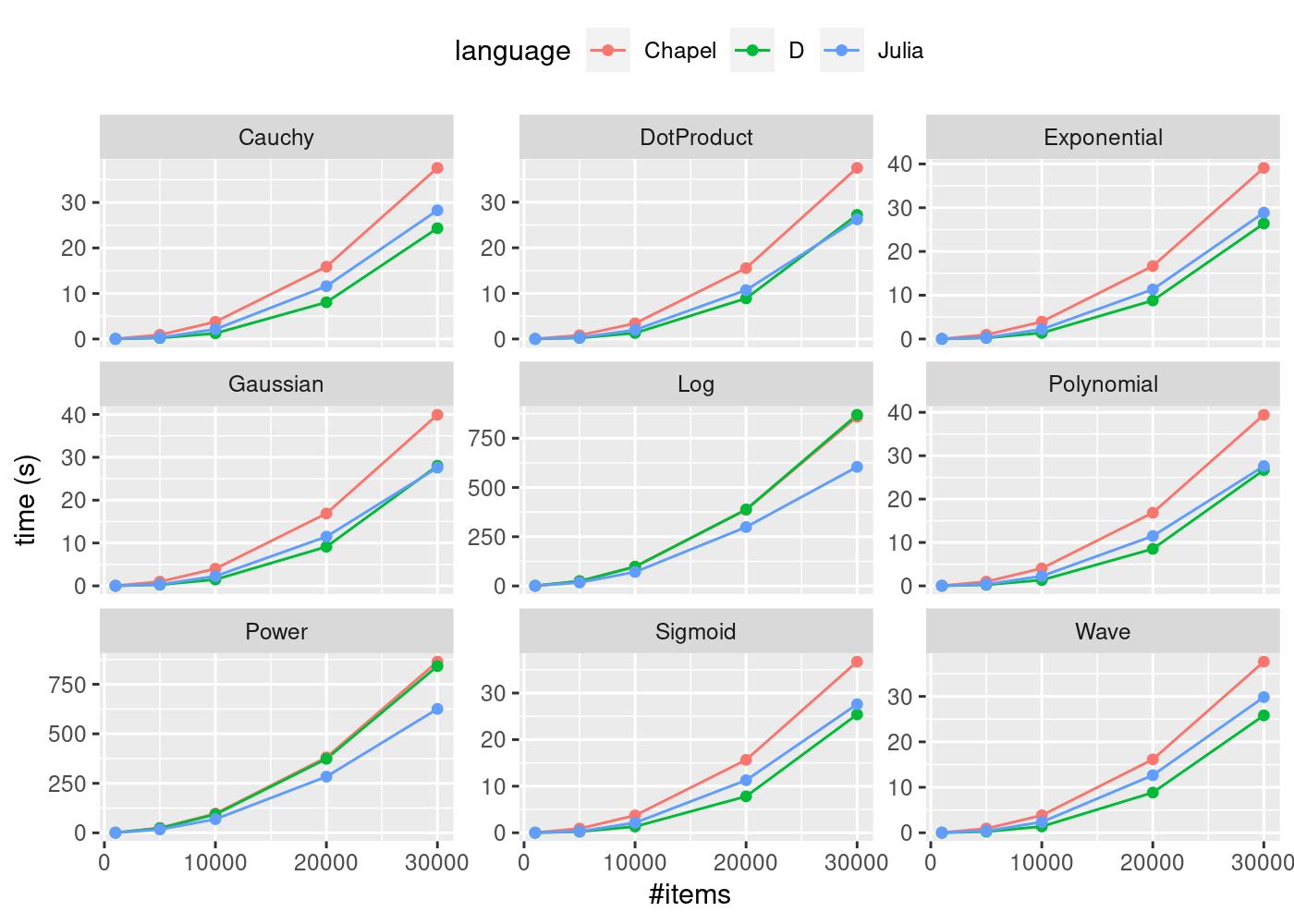
The above chart (generated using R’s ggplot2 using a script) shows the performance benchmark time taken against the number of items n for Chapel, D, and Julia, for nine kernels. D performs best in five of the nine kernels, Julia performs best in two of the nine kernels, and in two of the kernels (Dot and Gaussian) the picture is mixed. Chapel was the slowest for all of the kernel functions examined.

It is worth noting that the mathematics functions used in D were pulled from C’s math API made available in D through its core.stdc.math module because the mathematical functions in D’s standard library std.math can be quite slow. The math functions used are given here. By way of comparison, consider the mathdemo.d script comparing the imported C log function D’s log function from std.math:

$ ldc2 -O --boundscheck=off --ffast-math --mcpu=native --boundscheck=off mathdemo.d && ./mathdemo
Time taken for c log: 0.324789 seconds.
Time taken for d log: 2.30737 seconds.

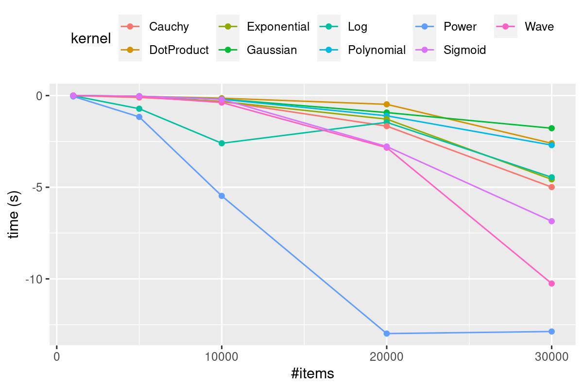
The Matrix object used in the D benchmark was implemented specifically because the use of modules outside standard language libraries was disallowed. To make sure that this implementation is competitive, i.e., it does not unfairly represent D’s performance, it is compared to Mir’s ndslice library written in D. The chart below shows matrix implementation times minus ndslice times; negative means that ndslice is slower, indicating that the implementation used here does not negatively represent D’s performance.

Environment

The code was run on a computer with an Ubuntu 20.04 OS, 32 GB memory, and an Intel® Core™ i9–8950HK CPU @ 2.90GHz with 6 cores and 12 threads.

$ julia --version
julia version 1.4.1
$ dmd --version
DMD64 D Compiler v2.090.1
ldc2 --version
LDC - the LLVM D compiler (1.18.0):
  based on DMD v2.088.1 and LLVM 9.0.0
$ chpl --version
chpl version 1.22.0

Compilation

Chapel:

chpl script.chpl kernelmatrix.chpl --fast && ./script

D:

ldc2 script.d kernelmatrix.d arrays.d -O5 --boundscheck=off --ffast-math -mcpu=native && ./script

Julia (no compilation required but can be run from the command line):

julia script.jl

Implementations

Efforts were made to avoid non-standard libraries while implementing these kernel functions. The reasons for this are:

  • To make it easy for the reader after installing the language to copy and run the code. Having to install external libraries can be a bit of a “faff”.
  • Packages outside standard libraries can go extinct, so avoiding external libraries keeps the article and code relevant.
  • It’s completely transparent and shows how each language works.

Chapel

Chapel uses a forall loop to parallelize over threads. Also, C pointers to each item are used rather than the default array notation, and guided iteration over indices is used:

proc calculateKernelMatrix(K, data: [?D] ?T)
{
  var n = D.dim(0).last;
  var p = D.dim(1).last;
  var E: domain(2) = {D.dim(0), D.dim(0)};
  var mat: [E] T;
  var rowPointers: [1..n] c_ptr(T) =
    forall i in 1..n do c_ptrTo(data[i, 1]);

  forall j in guided(1..n by -1) {
    for i in j..n {
      mat[i, j] = K.kernel(rowPointers[i], rowPointers[j], p);
      mat[j, i] = mat[i, j];
    }
  }
  return mat;
}

Chapel code was the most difficult to optimize for performance and required the highest number of code changes.

D

D uses a taskPool of threads from its std.parallel package to parallelize code. The D code underwent the fewest number of changes for performance optimization—a lot of the performance benefits came from the specific compiler used and the flags selected (discussed later). My implementation of a Matrix allows columns to be selected by reference via refColumnSelect.

auto calculateKernelMatrix(alias K, T)(K!(T) kernel, Matrix!(T) data)
{
  long n = data.ncol;
  auto mat = Matrix!(T)(n, n);

  foreach(j; taskPool.parallel(iota(n)))
  {
    auto arrj = data.refColumnSelect(j).array;
    foreach(long i; j..n)
    {
      mat[i, j] = kernel(data.refColumnSelect(i).array, arrj);
      mat[j, i] = mat[i, j];
    }
  }
  return mat;
}

Julia

The Julia code uses the @threads macro for parallelising the code and @views macro for referencing arrays. One confusing thing about Julia’s arrays is their reference status. Sometimes, as in this case, arrays will behave like value objects and they have to be referenced by using the @views macro, otherwise they generate copies. At other times they behave like reference objects, for example, when passing them into a function. It can be a little tricky dealing with this because you don’t always know what set of operations will generate a copy, but where this occurs @views provides a good solution.

The Symmetric type saves the small bit of extra work needed for allocating to both sides of the matrix.

function calculateKernelMatrix(Kernel::K, data::Array{T}) where {K <: AbstractKernel,T <: AbstractFloat}
  n = size(data)[2]
  mat = zeros(T, n, n)
  @threads for j in 1:n
      @views for i in j:n
          mat[i,j] = kernel(Kernel, data[:, i], data[:, j])
      end
  end
  return Symmetric(mat, :L)
end

The @bounds and @simd macros in the kernel functions were used to turn bounds checking off and apply SIMD optimization to the calculations:

struct DotProduct <: AbstractKernel end
@inline function kernel(K::DotProduct, x::AbstractArray{T, N}, y::AbstractArray{T, N}) where {T,N}
  ret = zero(T)
  m = length(x)
  @inbounds @simd for k in 1:m
      ret += x[k] * y[k]
  end
  return ret
end

These optimizations are quite visible but very easy to apply.

Memory Usage

The total time for each benchmark and the total memory used was captured using the /usr/bin/time -v command. The output for each of the languages is given below.

Chapel took the longest total time but consumed the least amount of memory (nearly 6GB RAM peak memory):

Command being timed: "./script"
	User time (seconds): 113190.32
	System time (seconds): 6.57
	Percent of CPU this job got: 1196%
	Elapsed (wall clock) time (h:mm:ss or m:ss): 2:37:39
	Average shared text size (kbytes): 0
	Average unshared data size (kbytes): 0
	Average stack size (kbytes): 0
	Average total size (kbytes): 0
	Maximum resident set size (kbytes): 5761116
	Average resident set size (kbytes): 0
	Major (requiring I/O) page faults: 0
	Minor (reclaiming a frame) page faults: 1439306
	Voluntary context switches: 653
	Involuntary context switches: 1374820
	Swaps: 0
	File system inputs: 0
	File system outputs: 8
	Socket messages sent: 0
	Socket messages received: 0
	Signals delivered: 0
	Page size (bytes): 4096
	Exit status: 0

D consumed the highest amount of memory (around 20GB RAM peak memory) but took less total time than Chapel to execute:

Command being timed: "./script"
	User time (seconds): 106065.71
	System time (seconds): 58.56
	Percent of CPU this job got: 1191%
	Elapsed (wall clock) time (h:mm:ss or m:ss): 2:28:29
	Average shared text size (kbytes): 0
	Average unshared data size (kbytes): 0
	Average stack size (kbytes): 0
	Average total size (kbytes): 0
	Maximum resident set size (kbytes): 20578840
	Average resident set size (kbytes): 0
	Major (requiring I/O) page faults: 0
	Minor (reclaiming a frame) page faults: 18249033
	Voluntary context switches: 3833
	Involuntary context switches: 1782832
	Swaps: 0
	File system inputs: 0
	File system outputs: 8
	Socket messages sent: 0
	Socket messages received: 0
	Signals delivered: 0
	Page size (bytes): 4096
	Exit status: 0

Julia consumed a moderate amount of memory (around 7.5 GB peak memory) but ran the quickest—probably because its random number generator is the fastest:

Command being timed: "julia script.jl"
	User time (seconds): 49794.85
	System time (seconds): 30.58
	Percent of CPU this job got: 726%
	Elapsed (wall clock) time (h:mm:ss or m:ss): 1:54:18
	Average shared text size (kbytes): 0
	Average unshared data size (kbytes): 0
	Average stack size (kbytes): 0
	Average total size (kbytes): 0
	Maximum resident set size (kbytes): 7496184
	Average resident set size (kbytes): 0
	Major (requiring I/O) page faults: 794
	Minor (reclaiming a frame) page faults: 38019472
	Voluntary context switches: 2629
	Involuntary context switches: 523063
	Swaps: 0
	File system inputs: 368360
	File system outputs: 8
	Socket messages sent: 0
	Socket messages received: 0
	Signals delivered: 0
	Page size (bytes): 4096
	Exit status: 0

Performance optimization

The process of performance optimization in all three languages was very different, and all three communities were very helpful in the process. But there were some common themes.

  • Static dispatching of kernel functions instead of using polymorphism. This means that when passing the kernel function, use parametric (static compile time) polymorphism rather than runtime (dynamic) polymorphism where dispatch with virtual functions carries a performance penalty.
  • Using views/references rather than copying data over multiple threads makes a big difference.
  • Parallelising the calculations makes a huge difference.
  • Knowing if your array is row/column major and using that in your calculation makes a huge difference.
  • Bounds checks and compiler optimizations make a tremendous difference, especially in Chapel and D.
  • Enabling SIMD in D and Julia made a contribution to the performance. In D this was done using the -mcpu=native flag, and in Julia this was done using the @simd macro.

In terms of language-specific issues, getting to performant code in Chapel was the most challenging, and the Chapel code changed the most from easy-to-read array operations to using pointers and guided iterations. But on the compiler side it was relatively easy to add --fast and get a large performance boost.

The D code changed very little, and most of the performance was gained by the choice of compiler and its optimization flags. D’s LDC compiler is rich in terms of options for performance optimization. It has 8 -O optimization levels, but some are repetitions of others. For instance, -O, -O3, and -O5 are identical, and there are myriad other flags that affect performance in various ways. In this case the flags used were -O5 --boundscheck=off –ffast-math, representing aggressive compiler optimizations, bounds checking, and LLVM’s fast-math, and -mcpu=native to enable CPU vectorization instructions.

In Julia the macro changes discussed previously markedly improved the performance, but they were not too intrusive. I tried changing the optimization -O level, but this did not improve performance.

Quality of life

This section examines the relative pros and cons around the convenience and ease of use of each language. People underestimate the effort it takes to use a language day-to-day; the support and infrastructure required is significant, so it is worth comparing various facets of each language. Readers seeking to avoid the TLDR should scroll to the end of this section for the table comparing the language features discussed here. Every effort has been made to be as objective as possible, but comparing programming languages is difficult, bias prone, and contentious, so read this section with that in mind. Some elements looked at, such as arrays, are from the “data science”/technical/scientific computing point of view, and others are more general.

Interactivity

Programmers want a fast code/compile/result loop during development to quickly observe results and outputs in order to make progress or necessary changes. Julia’s interpreter is hands down the best for this and offers a smooth and feature-rich development experience, and D comes a close second. This code/compile/result loop in compilers can be slow even when compiling small code volumes. D has three compilers, the standard DMD compiler, the LLVM-based LDC compiler, and the GCC-based GDC. In this development process, the DMD and LDC compilers were used. DMD has very fast compilation times which is great for development. The LDC compiler is great at creating fast code. Chapel’s compiler is very slow in comparison. To give an example, running Linux’s time command on DMD vs Chapel’s compiler for the kernel matrix code with no optimizations gives us for D:

real	0m0.545s
user	0m0.447s
sys	0m0.101s

Compared with Chapel:

real	0m5.980s
user	0m5.787s
sys	0m0.206s

That’s a large actual and psychological difference, it can make programmers reluctant to check their work and delay the development loop if they have to wait for outputs, especially when source code increases in volume and compilation times become significant.

It is worth mentioning, however, that when developing packages in Julia, compilation times can be very long, and users have noticed that when they load some packages ,compilation times can stretch. So the experience of the development loop in Julia could vary, but in this specific case the process was seamless.

Documentation and examples

One way of comparing documentation in the different languages is to compare them all with Python’s official documentation, which is the gold standard for programming languages. It combines examples with formal definitions and tutorials in a seamless and user-friendly way. Since many programmers are familiar with the Python documentation, this approach gives an idea of how they compare.

Julia’s documentation is the closest to Python’s documentation quality and gives the user a very smooth, detailed, and relatively painless transition into the language. It also has a rich ecosystem of blogs, and topics on many aspects of the language are easy to come by. D’s official documentation is not as good and can be challenging and frustrating, however there is a very good free book “Programming in D” which is a great introduction to the language, but no single book can cover a programming language and there are not many sources for advanced topics. Chapel’s documentation is quite good for getting things done, though examples vary in presence and quality. Often, the programmer needs a lot of knowledge to look in the right place. A good topic for comparison is file I/O libraries in Chapel, D, and Julia. Chapel’s I/O library has too few examples but is relatively clear and straightforward; D’s I/O is kind of spread across a few modules, and documentation is more difficult to follow; Julia’s I/O documentation has lots of examples and is clear and easy to follow.

Perhaps one factor affecting Chapel’s adoption is lack of example—since its arrays have a non-standard interface, the user has to work hard to become familiar with them. Whereas even though D’s documentation may not be as good in places, the language has many similarities to C and C++, so it gets away with more sparse documentation.

Multi-dimensional Array support

“Arrays” here does not refer to native C and C++ style arrays available in D, but mathematical arrays. Julia and Chapel ship with array support and D does not, but it has the Mir library which has multidimensional arrays (ndslice). In the implementation of kernel matrix, I wrote my own matrix object in D, which is not difficult if you understand the principle, but it’s not something a user wants to do. However, D has a linear algebra library called Lubeck which has impressive performance characteristics and interfaces with all the usual BLAS implementations. Julia’s arrays are by far the easiest and most familiar. Chapel’s arrays are more difficult to get started with than Julia’s but are designed to be run on single-core, multi-core, and computer clusters using the same or very similar code, which is a good unique selling point.

Language power

Since Julia is a dynamic programming language, some might say, “well Julia is a dynamic language which is far more permissive than static programming languages, therefore the debate is over”, but it’s more complicated than that. There is power in static type systems. Julia has a type system similar in nature to type systems from static languages, so you can write code as if you were using a static language, but you can do things reserved only for dynamic languages. It has a highly developed generic and meta-programming syntax and powerful macros. It also has a highly flexible object system and multiple dispatch. This mix of features is what makes Julia the most powerful language of the three.

D was intended to be a replacement for C++ and takes very much after C++ (and also borrows from Java), but makes template programming and compile-time evaluation much more user-friendly than in C++. It is a single dispatch language (though multi-methods are available in a package). Instead of macros, D has string and template “mixins” which serve a similar purpose.

Chapel has generic programming support and nascent support for single dispatch OOP, no macro support, and is not yet as mature as D or Julia in these terms.

Concurrency & Parallel Programming

Nowadays, new languages tout support for concurrency and its popular subset, parallelism, but the details vary a lot between languages. Parallelism is more relevant in this example and all three languages deliver. Writing parallel for loops is straightforward in all three languages.

Chapel’s concurrency model has much more emphasis on data parallelism but has tools for task parallelism and ships with support for cluster-based concurrency.

Julia has good support for both concurrency and parallelism.

D has industry strength support for parallelism and concurrency, though its support for threading is much less well documented with examples.

Standard Library

How good is the standard library of all three languages in general? What range of tasks do they allow users to easily tend to? It’s a tough question because library quality and documentation factor in. All three languages have very good standard libraries. D has the most comprehensive standard library, but Julia is a great second, then Chapel, but things are never that simple. For example, a user seeking to write binary I/O may find Julia the easiest to start with; it has the most straightforward, clear interface and documentation, followed by Chapel, and then D. Though in my implementation of an IDX file reader, D’s I/O was the fastest, but then Julia code was easy to write for cases unavailable in the other two languages.

Package Managers & Package Ecosystems

In terms of documentation, usage, and features, D’s Dub package manager is the most comprehensive. D also has a rich package ecosystem in the Dub website, Julia’s package manager runs tightly integrated with GitHub and is a good package system with good documentation. Chapel has a package manager but does not have a highly developed package ecosystem.

C Integration

C interop is easy in all three languages; Chapel has good documentation but is not as well popularised as the others. D’s documentation is better and Julia’s documentation is the most comprehensive. Oddly enough though, none of the languages’ documentation show the commands required to compile your own C code and integrate it with the language, which is an oversight especially when it comes to novices. It is, however, easy to search for and find examples for the compilation process in D and Julia.

Community

All three languages have convenient places where users can ask questions. For Chapel, the easiest place is Gitter, for Julia it’s Discourse (though there is a Julia Gitter), and for D it’s the official website forum. The Julia community is the most active, followed by D, and then Chapel. I’ve found that you’ll get good responses from all three communities, but you’ll probably get quicker answers from the D and Julia communities.

Chapel D Julia
Compilation/Interactivty Slow Fast Best
Documentation & Examples Detailed Patchy Best
Multi-dimensional Arrays Yes Native Only
(library support)
Yes
Language Power Good Great Best
Concurrency & Parallelism Great Great Good
Standard Library Good Great Great
Package Manager & Ecosystem Nascent Best Great
C Integration Great Great Great
Community Small Vibrant Largest

Table for quality of life features in Chapel, D & Julia

Summary

If you are a novice programmer writing numerical algorithms and doing calculations based in scientific computing and want a fast language that’s easy to use, Julia is your best bet. If you are an experienced programmer working in the same space, Julia is still a great option. If you specifically want a more conventional, “industrial strength”, statically compiled, high-performance language with all the “bells and whistles”, but want something more productive, safer, and less painful than C++, then D is your best bet. You can write “anything” in D and get great performance from its compilers. If you need to get array calculations happening on clusters, then Chapel is probably the easiest place to go.

In terms of raw performance on this task, D was the winner, clearly performing better in 5 out of the 9 kernels benchmarked. This exercise reveals that Julia’s label as a high-performance language is more than just hype—it has held it’s own against highly competitive languages. It was harder than expected to get competitive performance from Chapel—it took a lot of investigation from the Chapel team to come up with the current solution. However, as the Chapel language matures we could see further improvement.

Lomuto’s Comeback

The Continental Club in Austin, Texas, USA
Sunday, January 5, 1987

“Thank you for your kind invitation, Mr. Lomuto. I will soon return to England so this is quite timely.”

“And thanks for agreeing to meeting me, Mister… Sir… Charles… A.R… Hoare. It’s a great honor. I don’t even know how to address you. Were you knighted?”

“Call me Tony, and if it’s not too much imposition please allow me to call you Nico.”

On the surface, a banal scene—two men enjoying a whiskey. However, a closer look revealed a number of intriguing details. For starters, a tension you could cut with a knife.

Dressed in a perfectly tailored four-piece suit worn with the nonchalance only an Englishman could pull off, Tony Hoare was as British as a cup of tea. His resigned grimaces as he was sipping from his glass spoke volumes about his opinion of Bourbon versus Scotch. On the other side of the small table, Nico Lomuto couldn’t have been more different: a casually dressed coder enjoying his whiskey with Coca-Cola (a matter so outrageous that Tony had decided early on to studiously pretend not to notice, as he would when confronted with ripe body odor or an offensive tattoo), in a sort of relaxed awe at the sight of the Computer Science giant he had just met.

“Listen, Tony,” Nico said as the chit chat petered off, “about that partitioning algorithm. I never meant to publish or—”

“Oh? Yes, yes, the partitioning algorithm.” Tony’s eyebrows rose with feigned surprise, as if it had escaped his mind that every paper and book on quicksort in the past five years mentioned their names together. It was obviously the one thing connecting the two men and the motivation of the meeting, but Tony, the perfect gentleman, could talk about the weather for hours with a pink elephant in the room if his conversation partner didn’t bring it up.

“Yeah, that partitioning algorithm that keeps on getting mentioned together with yours,” Nico continued. “I’m not much of an algorithms theorist. I’m working on Ada, and this entire thing about my partition scheme is a distraction. The bothersome part about it”—Nico was speaking in the forthcoming tone of a man with nothing to hide—”is that it’s not even a better algorithm. My partitioning scheme will always do the same number of comparisons and at least as many swaps as yours. In the worst case, mine does n additional swaps—n! I can’t understand why they keep on mentioning the blessed thing. It’s out of my hands now. I can’t tell them what algorithms to teach and publish. It’s like bubblesort. Whenever anyone mentions quicksort, there’s some chowderhead—or should I say bubblehead—in the audience going, yes, I also heard of the bubblesort algorithm. Makes my blood curdle.”

Nico sighed. Tony nodded. Mutual values. Rapport filled the air in between as suddenly, quietly, and pleasantly as the smell of cookies out of the oven. A few seconds went by. Jack and Coke sip. On the other side of the table, Bourbon sip, resigned grimace.

Tony spoke with the carefully chosen words of a scientist who wants to leave no hypothesis unexplored. “I understand, Nico. Yet please consider the following. Your algorithm is simple and regular, moves in only one direction, and does at most one swap per step. That may be appropriate for some future machines that…”

“No matter the machine, more swaps can’t be better than fewer swaps. It’s common sense,” Nico said, peremptorily.

“I would not be so sure. Computers do not have common sense. Computers are surprising. It stands to reason they’ll continue to be. Well, how about we enjoy this evening. Nothing like a good conversation in a quiet club.”

“Yeah. Cheers. This is a fun place. I hear they’ll have live country music soon.”

“Charming.” Somewhat to his own surprise, Tony mustered a polite smile.

Chestnut Hill, Massachusetts, USA
Present Day

I’ve carried an unconfessed addiction to the sorting problem for many years. Wasn’t that difficult to hide—to a good extent, an obsessive inclination to studying sorting is a socially tolerated déformation professionnelle; no doubt many a programmer has spent a few late nights trying yet another sorting idea that’s going to be so much better than the others. So nobody raised an eyebrow when I wrote about sorting all the way back in 2002 (ever heard about “fit pivot?” Of course you didn’t). There was no intervention organized when I wrote D’s std.sort, which turned out to be sometimes quadratic (and has been thankfully fixed since). No scorn even when I wrote an academic paper on the selection problem (sort’s cousin) as an unaffiliated outsider, which even the conference organizers said was quite a trick. And no public outrage when I spoke about sorting at CppCon 2019. Coders understand.

So, I manage. You know what they say—one day at a time. Yet I did feel a tinge of excitement when I saw the title of a recent paper: “Branch Mispredictions Don’t Affect Mergesort.” Such an intriguing title. To start with, are branch mispredictions expected to affect mergesort? I don’t have much of an idea, mainly because everybody and their cat is using quicksort, not mergesort, so the latter hasn’t really been at the center of my focus. But hey, I don’t even need to worry about it because the title resolutely asserts that that problem I didn’t know I was supposed to worry about, I don’t need to worry about after all. So in a way the title cancels itself out. Yet I did read the paper (and recommend you do the same) and among many interesting insights, there was one that caught my attention: Lomuto’s partitioning scheme was discussed as a serious contender (against the universally-used Hoare partition) from an efficiency perspective. Efficiency!

It turns out modern computing architecture does, sometimes, violate common sense.

To Partition, Perchance to Sort

Let’s first recap the two partitioning schemes. Given an array and a pivot element, to partition the array means to arrange elements of the array such that all elements smaller than or equal to the pivot are on the left, and elements greater than or equal to the pivot are on the right. The final position of the pivot would be at the border. (If there are several equivalent pivot values that final pivot position may vary, with important practical consequences; for this discussion, however, we can assume that all array values are distinct.)

Lomuto’s partitioning scheme walks the array left to right maintaining a “read” position and a “write” position, both initially at 0. For each element read, if the value seen by the “read head” is greater than the pivot, it gets skipped (with the read head moving to the next position). Otherwise, the value at the read head is swapped with that at the write head, and both heads advance by one position. When the read head is done, the position of the write head defines the partition. Refer to the nice animation below (from Wikipedia user Mastremo, used unmodified under the CC-BY-SA 3.0 license).

The problem with Lomuto’s partition is that it may do unnecessary swaps. Consider the extreme case of an array with only the leftmost element greater than the pivot. That element will be awkwardly moved to the right one position per iteration step, in a manner not unlike, um, bubblesort.

Hoare’s partitioning scheme elegantly solves that issue by iterating concomitantly from both ends of the array with two “read/write heads”. They skip elements that are already appropriately placed (less than the pivot on the left, greater than the pivot on the right), and swap only one smaller element from the left with one greater element from the right. When the two heads meet, the array is partitioned around the meet point. The extreme case described above is handled with a single swap. Most contemporary implementations of quicksort use Hoare partition, for obvious reasons: it does as many comparisons as the Lomuto partition and fewer swaps.

Given that Hoare partition clearly does less work than Lomuto partition, the question would be why ever teach or use the latter at all. Alexander Stepanov, the creator of the STL, authored a great discussion about partitioning and makes a genericity argument: Lomuto partition only needs forward iterators, whereas Hoare partition requires bidirectional iterators. That’s a valuable insight, albeit of limited practical utility: yes, you could use Lomuto’s partition on singly-linked lists, but most of the time you partition for quicksort’s sake, and you don’t want to quicksort singly-linked lists; mergesort would be the algorithm of choice.

Yet a very practical—and very surprising—argument does exist, and is the punchline of this article: implemented in a branch-free manner, Lomuto partition is a lot faster than Hoare partition on random data. Given that quicksort spends most of its time partitioning, it follows that we are looking at a hefty improvement of quicksort (yes, I am talking about industrial strength implementations for C++ and D) by replacing its partitioning algorithm with one that literally does more work.

You read that right.

Time to Spin Some Code

To see how the cookie crumbles, let’s take a look at a careful implementation of Hoare partition. To eliminate all extraneous details, the code in this article is written for long as the element type and uses raw pointers. It compiles and runs the same with a C++ or D compiler. This article will carry along implementations of all routines in both languages because much research literature measures algorithm performance using C++’s std::sort as an important baseline.

/**
Partition using the minimum of the first and last element as pivot.
Returns: a pointer to the final position of the pivot.
*/
long* hoare_partition(long* first, long* last) {
    assert(first <= last);
    if (last - first < 2)
        return first; // nothing interesting to do
    --last;
    if (*first > *last)
        swap(*first, *last);
    auto pivot_pos = first;
    auto pivot = *pivot_pos;
    for (;;) {
        ++first;
        auto f = *first;
        while (f < pivot)
            f = *++first;
        auto l = *last;
        while (pivot < l)
            l = *--last;
        if (first >= last)
            break;
        *first = l;
        *last = f;
        --last;
    }
    --first;
    swap(*first, *pivot_pos);
    return first;
}

(You may find the choice of pivot a bit odd, but not to worry: usually it’s a more sophisticated scheme—such as median-of-3—but what’s important to the core loop is that the pivot is not the largest element of the array. That allows the core loop to omit a number of limit conditions without running off array bounds.)

There are a lot of good things to say about the efficiency of this implementation (which you’re likely to find, with minor details changed, in implementations of the C++ or D standard library). You could tell the code above was written by people who live trim lives. People who keep their nails clean, show up when they say they’ll show up, and call Mom regularly. They do a wushu routine every morning and don’t let computer cycles go to waste. That code has no slack in it. The generated Intel assembly is remarkably tight and virtually identical for C++ and D. It only varies across backends, with LLVM at a slight code size advantage (see clang and ldc) over gcc (see g++ and gdc).

The initial implementation of Lomuto’s partition shown below works well for exposition, but is sloppy from an efficiency perspective:

/**
Choose the pivot as the first element, then partition.
Returns: a pointer to the final position of the pivot. 
*/
long* lomuto_partition_naive(long* first, long* last) {
    assert(first <= last);
    if (last - first < 2)
        return first; // nothing interesting to do
    auto pivot_pos = first;
    auto pivot = *first;
    ++first;
    for (auto read = first; read < last; ++read) {
        if (*read < pivot) {
            swap(*read, *first);
            ++first;
        }
    }
    --first;
    swap(*first, *pivot_pos);
    return first;
}

For starters, the code above will do a lot of silly no-op swaps (array element with itself) if a bunch of elements on the left of the array are greater than the pivot. All that time first==write, so swapping *first with *write is unnecessary and wasteful. Let’s fix that with a pre-processing loop that skips the uninteresting initial portion:

/**
Partition using the minimum of the first and last element as pivot. 
Returns: a pointer to the final position of the pivot.
*/
long* lomuto_partition(long* first, long* last) {
    assert(first <= last);
    if (last - first < 2)
        return first; // nothing interesting to do
    --last;
    if (*first > *last)
        swap(*first, *last);
    auto pivot_pos = first;
    auto pivot = *first;
    // Prelude: position first (the write head) on the first element
    // larger than the pivot.
    do {
        ++first;
    } while (*first < pivot);
    assert(first <= last);
    // Main course.
    for (auto read = first + 1; read < last; ++read) {
        auto x = *read;
        if (x < pivot) {
            *read = *first;
            *first = x;
            ++first;
        }
    }
    // Put the pivot where it belongs.
    assert(*first >= pivot);
    --first;
    *pivot_pos = *first;
    *first = pivot;
    return first;
}

The function now chooses the pivot as the smallest of first and last element, just like hoare_partition. I also made another small change—instead of using the swap routine, let’s use explicit assignments. The optimizer takes care of that automatically (enregistering plus register allocation for the win), but expressing it in source helps us see the relatively expensive array reads and array writes. Now for the interesting part. Let’s focus on the core loop:

for (auto read = first + 1; read < last; ++read) {
    auto x = *read;
    if (x < pivot) {
        *read = *first;
        *first = x;
        ++first;
    }
}

Let’s think statistics. There are two conditionals in this loop: read < last and x < pivot. How predictable are they? Well, the first one is eminently predictable—you can reliably predict it will always be true, and you’ll only be wrong once no matter how large the array is. Compiler writers and hardware designers know this, and design the fastest path under the assumption loops will continue. (Gift idea for your Intel engineer friend: a doormat that reads “The Backward Branch Is Always Taken.”) The CPU will speculatively start executing the next iteration of the loop even before having decided whether the loop should continue. That work will be thrown away only once, at the end of the loop. That’s the magic of speculative execution.

Things are quite a bit less pleasant with the second test, x < pivot. If you assume random data and a randomly-chosen pivot, it could go either way with equal probability. That means speculative execution is not effective at all, which is very bad for efficiency. How bad? In a deeply pipelined architecture (as all are today), failed speculation means the work done by several pipeline stages needs to be thrown away, which in turn propagates a bubble of uselessness through the pipeline (think air bubbles in a garden hose). If these bubbles occur too frequently, the loop produces results at only a fraction of the attainable bandwidth. As the measurements section will show, that one wasted speculation takes away about 30% of the potential speed.

How to improve on this problem? Here’s an idea: instead of making decisions that control the flow of execution, we write the code in a straight-line manner and we incorporate the decisions as integers that guide the data flow by means of carefully chosen array indexing. Be prepared—this will force us to do silly things. For example, instead of doing two conditional writes per iteration, we’ll do exactly two writes per iteration no matter what. If the writes were not needed, we’ll overwrite words in memory with their own value. (Did I mention “silly things”?) To prepare the code for all that, let’s rewrite it as follows:

for (auto read = first + 1; read < last; ++read) {
    auto x = *read;
    if (x < pivot) {
        *read = *first;
        *first = x;
        first += 1; 
    } else {
        *read = x;
        *first = *first;
        first += 0; 
    }
}

Now the two branches of the loop are almost identical save for the data. The code is still correct (albeit odd) because on the else branch it needlessly writes *read over itself and *first over itself. How do we now unify the two branches? Doing so in an efficient manner takes a bit of pondering and experimentation. Conditionally incrementing first is easy because we can always write first += x < pivot. Piece of cake. The two memory writes are more difficult, but the basic idea is to take the difference between pointers and use indexing. Here’s the code. Take a minute to think it over:

for (; read < last; ++read) {
    auto x = *read;
    auto smaller = -int(x < pivot);
    auto delta = smaller & (read - first);
    first[delta] = *first;
    read[-delta] = x;
    first -= smaller;
}

To paraphrase a famous Latin aphorism, explanatio longa, codex brevis est. Short is the code, long is the ‘splanation. The initialization of smaller with -int(x < pivot) looks odd but has a good reason: smaller can serve as both an integral (0 or -1) used with the usual arithmetic and also as a mask that is 0 or 0xFFFFFFFF (i.e. bits set all to 0 or all to 1) used with bitwise operations. We will use that mask to allow or obliterate another integral in the next line that computes delta. If x < pivotsmaller is all ones and delta gets initialized to read - first. Subsequently, delta is used in first[delta] and read[-delta], which really are syntactic sugar for *(first + delta) and *(read - delta), respectively. If we substitute delta in those expressions, we obtain *(first + (read - first)) and *(read - (read - first)), respectively.

The last line, first -= smaller, is trivial: if x < pivot, subtract -1 from first, which is the same as incrementing first. Otherwise, subtract 0 from first, effectively leaving first alone. Nicely done.

With x < pivot substituted to 1, the calculation done in the body of the loop becomes:

auto x = *read;
int smaller = -1;
auto delta = -1 & (read - first);
*(first + (read - first)) = *first;
*(read - (read - first)) = x;
first -= -1;

Kind of magically the two pointer expressions simplify down to *read and *first, so the two assignments effect a swap (recall that x had been just initialized with *read). Exactly what we did in the true branch of the test in the initial version!

If x < pivot is false, delta gets initialized to zero and the loop body works as follows:

auto x = *read;
int smaller = 0;
auto delta = 0 & (read - first);
*(first + 0) = *first;
*(read - 0) = x;
first -= 0;

This time things are simpler: *first gets written over itself, *read also gets written over itself, and first is left alone. The code has no effect whatsoever, which is exactly what we wanted.

Let’s now take a look at the entire function:

long* lomuto_partition_branchfree(long* first, long* last) {
    assert(first <= last);
    if (last - first < 2)
        return first; // nothing interesting to do
    --last;
    if (*first > *last)
        swap(*first, *last);
    auto pivot_pos = first;
    auto pivot = *first;
    do {
        ++first;
        assert(first <= last);
    } while (*first < pivot);
    for (auto read = first + 1; read < last; ++read) {
        auto x = *read;
        auto smaller = -int(x < pivot);
        auto delta = smaller & (read - first);
        first[delta] = *first;
        read[-delta] = x;
        first -= smaller;
    }
    assert(*first >= pivot);
    --first;
    *pivot_pos = *first;
    *first = pivot;
    return first;
}

A beaut, isn’t she? Even more beautiful is the generated code—take a look at clang/ldc and g++/gdc. Again, there is a bit of variation across backends.

Experiments and Results

All code is available at https://github.com/andralex/lomuto.

To draw a fair comparison between the two partitioning schemes, I’ve put together a quicksort implementation. This is because most often a partition would be used during quicksort. For the sake of simplification, the test implementation omits a few details present in industrial quicksort implementations, which need to worry about a variety of data shapes (partially presorted ascending or descending, with local patterns, with many duplicates, etc). Library implementations choose the pivot carefully from a sample of usually 3-9 elements, possibly with randomization, and have means to detect and avoid pathological inputs, most often by using Introsort.

In our benchmark, for simplicity, we only test against random data, and the choice of pivot is simply the minimum of first and last element. This is without loss of generality; better pivot choices and adding introspection are done the same way regardless of the partitioning method. Here, the focus is to compare the performance of Hoare vs. Lomuto vs. branch-free Lomuto.

The charts below plot the time taken by one sorting operation depending on the input size. The machine used is an Intel i7-4790 at 3600 MHz with a 256KB/1MB/8MB cache hierarchy running Ubuntu 20.04. All builds were for maximum speed (-O3, no assertions, no boundcheck for the D language). The input is a pseudorandom permutation of longs with the same seed for all languages and platforms. To eliminate noise, the minimum is taken across several epochs.

The results for the D language are shown below, including the standard library’s std.sort as a baseline.

Chart by Visualizer
Chart by Visualizer

The results for C++ are shown in the plots below. Again the standard library implementation std::sort is included as a baseline.

Chart by Visualizer
Chart by Visualizer

One important measurement is the CPU utilization efficiency, shown by Intel VTune as “the micropipe”, a diagram illustrating inefficiencies in resource utilization. VTune’s reports are very detailed but the micropipe gives a quick notion of where the work goes. To interpret a micropipe, think of it as a funnel. The narrower the exit (on the right), the slower the actual execution as a fraction of potential speed.

The micropipes shown below correspond to the Hoare partition, Lomuto partition (in the traditional implementation), and branch-free Lomuto partition. The first two throw away about 30% of all work as bad speculation. In contrast, the Lomuto branchless partition wastes no work on speculation, which allows it a better efficiency in spite of more memory writes.
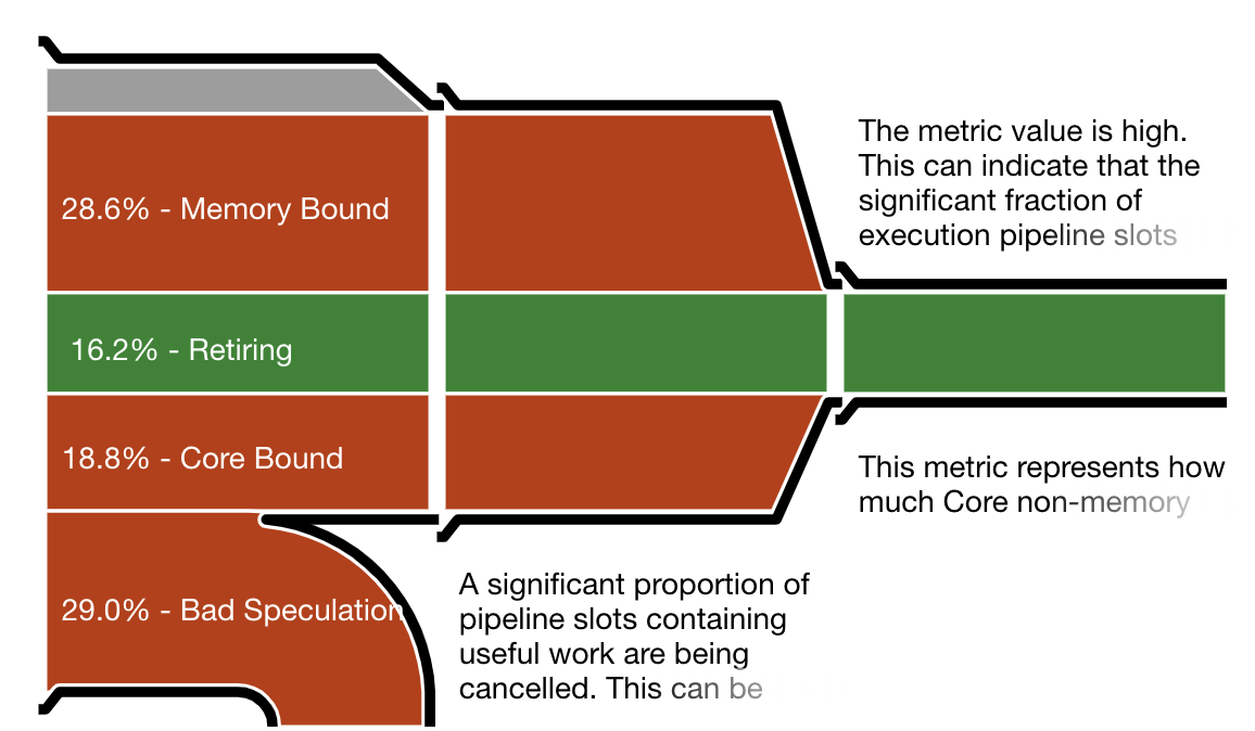
Intel VTune pipe efficiency diagram for the Hoare partition. A large percentage of work is wasted on failed speculation.
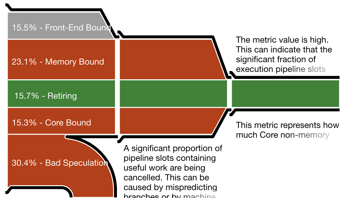
Intel VTune pipe efficiency diagram for the traditional “branchy” Lomuto partition, featuring about as much failed speculation as the Hoare partition.
Intel VTune pipe efficiency diagram for the Lomuto branch-free partition. Virtually no work is wasted on failed speculation, leading to a much better efficiency.

Discussion

The four versions (two languages times two backends) exhibit slight variations due to differences in standard library implementations and backend versions. It is not surprising that minute variations in generated code are liable to create measurable differences in execution speed.

As expected, the “branchy” Lomuto partition compares poorly with Hoare partition, especially for large input sizes. Both are within the same league as the standard library implementation of the sort routine. Sorting using the branchless Lomuto partition, however, is the clear winner by a large margin regardless of platform, backend, and input size.

It has become increasingly clear during the past few years that algorithm analysis—and proposals for improvements derived from it—cannot be done solely with pen and paper using stylized computer architectures with simplistic cost models. The efficiency of sorting is determined by a lot more than counting the comparisons and swaps—at least, it seems, the predictability of comparisons must be taken into account. In the future, I am hopeful that better models of computation will allow researchers to rein in the complexity. For the time being, it seems, algorithm optimization remains hopelessly experimental.

For sorting in particular, Lomuto is definitely back and should be considered by industrial implementations of quicksort on architectures with speculative execution.

Acknowledgments

Many thanks are due to Amr Elmasry, Jyrki Katajainen, and Max Stenmark for an inspirational paper. I haven’t yet been able to engineer a mergesort implementation (the main result of their paper) that beats the best quicksort described here, but I’m working on it. (Sorry, Sorters Anonymous… I’m still off the wagon.) I’d like to thank to Michael Parker and the commentators at the end of this post for fixing many of my non-native-speaker-isms. (Why do they say “pretend not to notice” and “pretend to not notice”? I never remember the right one.) Of course, most of the credit is due to Nico Lomuto, who defined an algorithm that hasn’t just stood the test of time—it passed it.

Interfacing D with C: Arrays and Functions (Arrays Part 2)

Digital Mars D logo

This post is part of an ongoing series on working with both D and C in the same project. The previous post explored the differences in array declaration and initialization. This post takes the next step: declaring and calling C functions that take arrays as parameters.

Arrays and C function declarations

Using C libraries in D is extremely easy. Most of the time, things work exactly as one would expect, but as we saw in the previous article there can be subtle differences. When working with C functions that expect arrays, it’s necessary to fully understand these differences.

The most straightforward and common way of declaring a C function that accepts an array as a parameter is to to use a pointer in the parameter list. For example, this hypothetical C function:

void f0(int *arr);

In C, any array of int can be passed to this function no matter how it was declared. Given int a[], int b[3], or int *c, the function calls f0(a), f0(b), and f0(c) are all the same: a pointer to the first element of each array is passed to the function. Or using the lingo of C programmers, arrays decay to pointers

Typically, in a function like f0, the implementer will expect the array to have been terminated with a marker appropriate to the context. For example, strings in C are arrays of char that are terminated with the \0 character (we’ll look at D strings vs. C strings in a future post). This is necessary because, without that character, the implementation of f0 has no way to know which element in the array is the last one. Sometimes, a function is simply documented to expect a certain length, either in comments or in the function name, e.g., a vector3f_add(float *vec) will expect that vec points to exactly 3 elements. Another option is to require the length of the array as a separate argument:

void f1(int *arr, size_t len);

None of these approaches is foolproof. If f0 receives an array with no end marker or which is shorter than documented, or if f1 receives an array with an actual length shorter than len, then the door is open for memory corruption. D arrays take this possibility into account, making it much easier to avoid such problems. But again, even D’s safety features aren’t 100% foolproof when calling C functions from D.

There are other, less common, ways array parameters may be declared in C:

void f2(int arr[]);
void f3(int arr[9]);
void f4(int arr[static 9]);

Although these parameters are declared using C’s array syntax, they boil down to the exact same function signature as f0 because of the aforementioned pointer decay. The [9] in f3 triggers no special enforcement by the compiler; arr is still effectively a pointer to int with unknown length. The [9] serves as documentation of what the function expects, and the implementation cannot rely on the array having nine elements.

The only potential difference is in f4. The static added to the declaration tells the compiler that the function must take an array of, in this case, at least nine elements. It could have more than nine, but it can’t have fewer. That also rules out null pointers. The problem is, this isn’t necessarily enforced. Depending on which C compiler you use, if you shortchange the function and send it less than nine elements you might see warnings if they are enabled, but the compiler might not complain at all. (I haven’t tested current compilers for this article to see if any are actually reporting errors for this, or which ones provide warnings.)

The behavior of C compilers doesn’t matter from the D side. All we need be concerned with is declaring these functions appropriately so that we can call them from D such that there are no crashes or unexpected results. Because they are all effectively the same, we could declare them all in D like so:

extern(C):
void f0(int* arr);
void f1(int* arr, size_t len);
void f2(int* arr);
void f3(int* arr);
void f4(int* arr);

But just because we can do a thing doesn’t mean we should. Consider these alternative declarations of f2, f3, and f4:

extern(C):
void f2(int[] arr);
void f3(int[9] arr);
void f4(int[9] arr);

Are there any consequences of taking this approach? The answer is yes, but that doesn’t mean we should default to int* in each case. To understand why, we need first to explore the innards of D arrays.

The anatomy of a D array

The previous article showed that D makes a distinction between dynamic and static arrays:

int[] a0;
int[9] a1;

a0 is a dynamic array and a1 is a static array. Both have the properties .ptr and .length. Both may be indexed using the same syntax. But there are some key differences between them.

Dynamic arrays

Dynamic arrays are usually allocated on the heap (though that isn’t a requirement). In the above case, no memory for a0 has been allocated. It would need to be initialized with memory allocated via new or malloc, or some other allocator, or with an array literal. Because a0 is uninitialized, a0.ptr is null and a0.length is 0.

A dynamic array in D is an aggregate type that contains the two properties as members. Something like this:

struct DynamicArray {
    size_t length;
    size_t ptr;
}

In other words, a dynamic array is essentially a reference type, with the pointer/length pair serving as a handle that refers to the elements in the memory address contained in the ptr member. Every built-in D type has a .sizeof property, so if we take a0.sizeof, we’ll find it to be 8 on 32-bit systems, where size_t is a 4-byte uint, and 16 on 64-bit systems, where size_t is an 8-byte ulong. In short, it’s the size of the handle and not the cumulative size of the array elements.

Static arrays

Static arrays are generally allocated on the stack. In the declaration of a1, stack space is allocated for nine int values, all of which are initialized to int.init (which is 0) by default. Because a1 is initialized, a1.ptr points to the allocated space and a1.length is 9. Although these two properties are the same as those of the dynamic array, the implementation details differ.

A static array is a value type, with the value being all of its elements. So given the declaration of a1 above, its nine int elements indicate that a1.sizeof is 9 * int.sizeof, or 36. The .length property is a compile-time constant that never changes, and the .ptr property, though not readable at compile time, is also a constant that never changes (it’s not even an lvalue, which means it’s impossible to make it point somewhere else).

These implementation details are why we must pay attention when we cut and paste C array declarations into D source modules.

Passing D arrays to C

Let’s go back to the declaration of f2 in C and give it an implementation:

void f2(int arr[]) {
    for(int i=0; i<3; ++i)
        printf("%d\n", arr[i]);
}

A naïve declaration in D:

extern(C) void f2(int[]);

void main() {
    int[] a = [10, 20, 30];
    f2(a);
}

I say naïve because this is never the right answer. Compiling f2.c with df2.d on Windows (cl /c f2.c in the “x64 Native Tools” command prompt for Visual Studio, followed by dmd -m64 df2.d f2.obj), then running df2.exe, shows me the following output:

3
0
1970470928

There is no compiler error because the declaration of f2 is pefectly valid D. The extern(C) indicates that this function uses the cdecl calling convention. Calling conventions affect the way arguments are passed to functions and how the function’s symbol is mangled. In this case, the symbol will be either _f2 or f2 (other calling conventions, like stdcallextern(Windows) in D—have different mangling schemes). The declaration still has to be valid D. (In fact, any D function can be marked as extern(C), something which is necessary when creating a D library that will be called from other languages.)

There is also no linker error. DMD is calling out to the system linker (in this case, Microsoft’s link.exe), the same linker used by the system’s C and C++ compilers. That means the linker has no special knowledge about D functions. All it knows is that there is a call to a symbol, f2 or _f2, that needs to be linked with the implementation. Since the type and number of parameters are not mangled into the symbol name, the linker will happily link with any matching symbol it finds (which, by the way, is the same thing it would do if a C program tried to call a C function which was declared with an incorrect parameter list).

The C function is expecting a single pointer as an argument, but it’s instead receiving two values: the array length followed by the array pointer.

The moral of this story is that any C function with array parameters declared using array syntax, like int[], should be declared to accept pointers in D. Change the D source to the following and recompile using the same command line as before (there’s no need to recompile the C file):

extern(C) void f2(int*);

void main() {
    int[] a = [10, 20, 30];
    f2(a.ptr);
}

Note the use of a.ptr. It’s an error to try to pass a D array argument where a pointer is expected (with one very special exception, string literals, which I’ll cover in the next article in this series), so the array’s .ptr property must be used instead.

The story for f3 and f4 is similar:

void f3(int arr[9]);
void f4(int arr[static 9]);

Remember, int[9] in D is a static array, not a dynamic array. The following do not match the C declarations:

void f3(int[9]);
void f4(int[9]);

Try it yourself. The C implementation:

void f3(int arr[9]) {
    for(int i=0; i<9; ++i)
        printf("%d\n", arr[i]);
}

And the D implementation:

extern(C) void f3(int[9]);

void main() {
    int[9] a = [10, 20, 30, 40, 50, 60, 70, 80, 90];
    f3(a);
}

This is likely to crash, depending on the system. Rather than passing a pointer to the array, this code is instead passing all nine array elements by value! Now consider a C library that does something like this:

typedef float[16] mat4f;
void do_stuff(mat4f mat);

Generally, when writing D bindings to C libraries, it’s a good idea to keep the same interface as the C library. But if the above is translated like the following in D:

alias mat4f = float[16];
extern(C) void do_stuff(mat4f);

The sixteen floats will be passed to do_stuff every time it’s called. The same for all functions that take a mat4f parameter. One solution is just to do the same as in the int[] case and declare the function to take a pointer. However, that’s no better than C, as it allows the function to be called with an array that has fewer elements than expected. We can’t do anything about that in the int[] case, but that will usually be accompanied by a length parameter on the C side anyway. C functions that take typedef’d types like mat4f usually don’t have a length parameter and rely on the caller to get it right.

In D, we can do better:

void do_stuff(ref mat4f);

Not only does this match the API implementor’s intent, the compiler will guarantee that any arrays passed to do_stuff are static float arrays with 16 elements. Since a ref parameter is just a pointer under the hood, all is as it should be on the C side.

With that, we can rewrite the f3 example:

extern(C) void f3(ref int[9]);

void main() {
    int[9] a = [10, 20, 30, 40, 50, 60, 70, 80, 90];
    f3(a);
}

Conclusion

Most of the time, when interfacing with C from D, the C API declarations and any example code can be copied verbatim in D. But most of the time is not all of the time, so care must be taken to account for those exceptional cases. As we saw in the previous article, carelessness when declaring array variables can usually be caught by the compiler. As this article shows, the same is not the case for C function declarations. Interfacing D with C requires the same care as when writing C code.

In the next article in this series, we’ll look at mixing D strings and C strings in the same program and some of the pitfalls that may arise. In the meantime, Steven Schveighoffer’s excellent article, “D Slices”, is a great place to start for more details about D arrays.

Thanks to Walter Bright and Átila Neves for their valuable feedback on this article.

DustMite: The General-Purpose Data Reduction Tool

If you’ve been around for a while, or are a particularly adventurous developer who enjoys mixing language features in interesting ways, you may have run into one compiler bug or two:

Implementation bugs are inevitably a part of using cutting-edge programming languages. Should you run into one, the steps to proceed are generally as follows:

  1. Reduce the failing program to a minimal, self-contained example.
  2. Add a description of what happens and what you expect to happen.
  3. Post it on the bug tracker.

Nine years ago, an observation was made that when filing and fixing compiler bugs, a disproportionate amount of time was spent on the first step. When your program stops compiling “out of the blue”, or when the bug stops reproducing after the code is taken out of its context, manually paring down a large codebase by repeatedly cutting out code and checking if the bug still occurs becomes a tedious and repetitive task.

Fortunately, tedious and repetitive tasks are what computers are good for; they just have to be tricked into doing them, usually by writing a program. Enter DustMite.


The first version.

The basic operation is simple. The tool takes as inputs:

  • a data set to reduce (such as, a directory containing D source code which exhibits a particular compiler bug)
  • an oracle (or, more mundanely, a test script), which itself:
  • takes as input a variation of the data set, and
  • produces a yes-or-no answer on whether the input still satisfies the sought property (such as reproducing the particular compiler bug).

DustMite’s output is some local minimum variation of the data set, which it reaches by consecutively trying to remove parts of the data set and saving the results which the oracle approves. In the compiler bug example, this means removing bits of code which are not required to reproduce the problem at hand.

DustMite wouldn’t be very efficient if it attempted to remove things line-by-line or character-by-character. In order to maximize the chance of finding good reductions, the input is parsed into a tree according to the syntax of the input files.

Each tree node consists of a “head” (string), children (list of node pointers), and “tail” (string). Technically, it is redundant to have both “head” and “tail”, but they make representing some constructs and performing reductions much simpler, such as paren/bracket pairs.


Nodes are arranged into a binary tree as an optimization.

Additionally, nodes may have a list of dependencies. The dependency relationship essentially means “if this node is removed, these nodes should be removed too”. These constraints are not representable using just the tree structure described above, and are used to allow reducing things such as lists where trailing item delimiters are not allowed, or removing a function parameter and corresponding arguments from the entire code base at once.

In the case of D source code, declarations, statements, and subexpressions get their own tree nodes, so that they can be removed in one go if unneeded. The parser DustMite uses for D source code is intentionally very simple because it needs to handle potentially invalid D code, and you don’t want your bug reduction tool to also crash on top of the compiler.


How DustMite sees a simple D program.

An algorithm decides the order in which nodes are queued for potential deletion; DustMite implements several (it calls them “strategies”). Fundamentally, a strategy’s interface is (statei, resulti) ⇒ (statei+1, reductioni+1), i.e., which reduction is chosen next depends on the previous reduction and its result. The default “inbreadth” strategy visits nodes in ascending depth order (row by row) and starts over from the top as long as it finds new reductions.

DustMite today supports quite a few more options:


The current version.

Probably, the most interesting of these is the -j switch—one reason being that DustMite’s task is inherently not parallelizable. Which reduction is chosen next, and the tree version to which that reduction is applied, depends on the previous reduction’s result.

DustMite works around this by putting unused CPU cores to work on lookahead: using a highly sophisticated predictor, it guesses what the result of the current reduction will be, and based on that assumption, calculates the next reduction. If the guess was right, great! We get to use that result. Otherwise, the work is wasted. Implementing this meant that strategies now needed to have copyable state, and so had to be refactored from an imperative style to a state machine.

Unfortunately, although the highly expected feature was implemented four years ago, the initial implementation was rather underwhelming. DustMite still did too much work in the main thread and wasted too much CPU time on rescanning the data set tree on every reduction. The problem was so bad that, at high core counts, lookahead mode was even slower than single-threaded mode.

I have recently set out to resolve these inadequacies. The following obstacles stood in the way:

Problem 1: Hashing was too slow. Because the oracle’s services (i.e., running the test script) are usually expensive, DustMite keeps track of a cache of previously attempted reductions and their outcome. This helps because not all tree transformations result in a change of output, and some strategies will retry reductions in successive iterations. A hash of the tree is used as the cache key; however, calculating it requires walking the entire tree every time, which is slow for large inputs.

Would it be possible to make the hash calculation incremental? One approach would be Merkle trees (each node’s hash is the hash of its children’s hashes), however that is suboptimal in the case of e.g., empty leaf nodes. CS erudite Ivan Kazmenko blesses us with an answer: polynomial hashes! By representing strings as polynomials, it is possible to use modulo arithmetic to calculate an incremental fixed-size hash and cache subtree hashes per node.


Each node holds its cumulative hash and length.

The number theory staggered me at first, so I recruited the assistance of feep from #d. After we went through a few draft implementations, I could begin working on the final version. The first improvement was replacing the naive exponentiation algorithm with exponentiation by squaring (D CTFE allowed precomputing a table at compile-time and a faster calculation than the classical method). Next, there was the matter of the modulo.

Initially, we used integer overflow for modulo arithmetic (i.e. q=264), however Ivan cautioned against using powers of two as the modulo, as this makes the algorithm susceptible to Thue-Morse strings. Not long ago I was experimenting with using long multiplication/division CPU instructions (where multiplying one machine word by another yields the result in two machine words with a high and low part, and vice-versa for division). D allows generating assembler code specific to the types that the function template is instantiated with, though in DustMite we only use the unsigned 64-bit variant (on x86 we fall back to using integer overflow).

With the hashing algorithm implemented, all that remained was to mark dirty nodes (they or their children had their content edited) and incrementally recalculate their hashes as needed. Dependencies posed a small obstacle: at the time, they were implemented as simply an array of pointers to the dependency node within the tree. As such, we didn’t know how to get to their parents (to mark them dirty as well), however this was easily overcome by adding a “parent” pointer to each node.

Well, or so I thought, until I got to work on the next problem.

Problem 2: Copying the tree. At the time, the current version of the tree representing the data set was part of the global state. Because of this, applying a reduction was implemented twice:

This was clumsy, but faster and less complicated than making a copy of the entire tree just to change one part of it to test a reduction. However, doing so was a requirement for proper lookahead, otherwise we would be unable to test reductions based on results where past tests predicted a positive outcome, or do nearly anything in a separate thread.

One issue was the tree “internal pointers”—making a copy would require updating all pointers within the tree to point to the new copies in the new tree. This was easy for children/parent pointers (since we can reliably visit every such pointer exactly once), but not quite for dependencies: because they were also implemented as simple pointers to nodes, we would have to keep track of a map of which node was copied where in order to update the dependency pointers.

One way to solve this would be to change the representation of node references from pointers to indices into a node array; this way, copying the tree would be as simple as a .dup. However, large inputs meant many nodes, and I wanted to see if it was possible to avoid iterating over every node in the tree (i.e. O(n)) for every reduction.

Was it possible? It would mean that we would copy only the modified nodes and their parents, leaving the rest of the tree in-place, and only reusing it as the copies’ children. This goal conflicted with the existence of “parent” pointers, because a parent would have to point towards either the old or new root, so to resolve this ambiguity every node would have to be copied. As a result, the way we handled dependencies needed to be rethought.


Editing trees with “copy on write” involves copying just the edited nodes (🔴), and their parents.

With internal pointers out, the next best thing to array indices for referencing a node was a series of instructions for how to reach the node from the tree root: an address. The representation of these addresses that I chose was a bit string represented as a linked list, where each list node holds the child index at that depth, starting from the deep end. Such a representation can be arranged in a tree where the root-side ends are shared, mimicking the structure of the tree containing the nodes for the reduced data, and thus allowing us to reuse memory and minimize allocations.


Nodes cannot hold their own address (as that would make them unmovable),
which is why they need to be stored outside of the main tree.

For addresses to work, the object they point at needs to remain the same, which means that we can no longer simply remove children from tree nodes—an address going through the second child would become invalid if the first child was removed. Rewriting all affected addresses for every tree edit is, of course, impractical, which leads us to the introduction of tombstones—dead nodes that only serve to preserve the index of the children that follow it. Because one of the possible reduction types involves moving subtrees around the tree, we now also have “redirects” (which are just tombstones with a “see here” address attached).

With the above changes in place, we can finally move forward with fixing and optimizing lookahead, as well as implementing incremental rehashing in a way that’s compatible with the above! The mutable global “current” tree variable is gone, save now simply takes a tree root as an argument, and applyReduction is now:

/// Apply a reduction to this tree, and return the resulting tree.
/// The original tree remains unchanged.
/// Copies only modified parts of the tree, and whatever references them.
Entity applyReduction(Entity origRoot, ref Reduction r)

With the biggest hurdle behind us, and a few more rounds of applying Walter Bright’s secret weapon, the performance metrics started to look more like what they should:


Going deeper would likely involve using OS-specific I/O APIs or rewriting D’s GC.

A mere 3.5x speed-up from a 32-fold increase in computational power may seem underwhelming. Here are some reasons for this:

  • With a 50/50 predictor, predictions form a complete binary tree, so doubling the number of parallel jobs gives you +1x more speed. That’s roughly log₂(jobs)-1, or 4 for 32 jobs – not far off!

  • The results will depend on the reduction being performed, so YMMV. For a certain artificial test case, one optimization (not pictured above) yielded a 500x speed-up!

  • DustMite does not try to keep all CPU cores busy all the time. If a prediction turns out false, all lookahead jobs based on it become wasted work, so DustMite only starts new lookahead tasks when a reduction’s outcome is resolved. Perhaps ideally DustMite would keep starting new jobs but kill them as soon as it discovers they’re based on a misprediction. As there is no cross-platform process group management in Phobos, the D standard library, this is something I left for future versions.

  • Some work is still done in the main thread, because moving it to a worker thread actually makes things slower due to the global GC lock.

There still remains one last place where DustMite iterates over every tree node per reduction: saving the tree to disk (so that it could be read by the test script). This seems unavoidable at first, but could actually be avoided by caching each node’s full text contents within the node itself.

I opted to leave this one out. With the other related improvements, such as using lockingBinaryWriter and aggregating writes of contiguous strings as one I/O operation, the increase in memory usage was much more dramatic than the decrease in execution time, even when optimized to just one allocation per reduction (polynomial hashing gives us every node’s total length for free). But, for a brief instant, DustMite processed reductions in sub-O(n) time.

One more addition is worth mentioning: Andrej Mitrovic suggested a switch which would replace removed text with whitespace, which would allow searching for exact line numbers in the test script. At the time, its addition posed significant challenges, as there needed to be some way to keep removed nodes in the tree but exclude them from future removal attempts. With the new tree representation, this became much easier, and also allowed creating the following animation:

In conclusion, I’d like to bring up that DustMite is good at more than just reducing compiler test cases. The wiki lists some ideas:

  • Finding the source of ambiguous or misleading compiler error messages (e.g., errors with the file/line information pointing only inside the standard library).

  • Alternative (much slower, but also much more thorough) method of verifying unit test code coverage. Just because a line of code is executed, that doesn’t mean it’s necessary; DustMite can be made to remove all code that does not affect the execution of your unit tests.

  • Similarly, if you have complete test coverage, it can be used for reducing the source tree to a minimal tree which includes support for only enabled unittests. This can be used to create a version of a program or library with a test-defined subset of features.

  • The --obfuscate mode can obfuscate your code’s identifiers. It can be used for preparing submission of proprietary code to bug trackers.

  • The --fuzz mode (a new feature) can help find bugs in compilers and tools by creating random programs (using fragments of other programs as input).

But DustMite is not limited to D programs (or any kind of programs) as input. With the --split option, we can tell DustMite how to parse and reduce other kinds of files. DustMite successfully handled the following scenarios:

  • reducing C++ programs (the D parser supports some C++-only syntax too);

  • reducing Python programs (using the indent split mode);

  • reducing a large commit to a minimal diff (using the diff split mode);

  • reducing a commit list, when git bisect is insufficient due to the problem being introduced across more than any single commit;

  • reducing a large data set to a minimal one, resulting in the same code coverage, with the purpose of creating a test suite;

  • and many more which I do not remember.

Today, some version of DustMite is readily available in major distributions (usually as part of some D-related package), so I’m happy having a favorite tool one apt-get / pacman -S away when I’m not at my PC.

Discovering a problem which can be elegantly reduced away by DustMite is always exciting for me, and I’m hoping you will find it useful too.