Category Archives: Code

A Pattern for Head-mutable Structures

When Andrei Alexandrescu introduced ranges to the D programming language, the gap between built-in and user-defined types (UDTs) narrowed, enabling new abstractions and greater composability. Even today, though, UDTs are still second-class citizens in D. One example of this is support for head mutability—the ability to manipulate a reference without changing the referenced value(s). This document details a pattern that will further narrow the UDT gap by introducing functions for defining and working with head-mutable user-defined types.

Introduction

D is neither Kernel nor Scheme—it has first-class and second-class citizens. Among its first-class citizens are arrays and pointers. One of the benefits these types enjoy is implicit conversion to head-mutable. For instance, const(T[]) is implicitly convertible to const(T)[]. Partly to address this difference, D has many ways to define how one type may convert to or behave like another – alias this, constructors, opDispatch, opCast, and, of course, subclassing. The way pointers and dynamic arrays decay into their head-mutable variants is different from the semantics of any of these features, so we would need to define a new type of conversion if we were to mimic this behavior.

Changing the compiler and the language to permit yet another way of converting one type into another is not desirable: it makes the job harder for compiler writers, makes an already complex language even harder to learn, and any implicit conversion can make code harder to read and maintain. If we can define conversions to head-mutable data structures without introducing compiler or language changes, this will also make the feature available to users sooner, since such a mechanism would not necessarily require changes in the standard library, and users could gradually implement it in their own code and benefit from the code in the standard library catching up at a later point.

Unqual

The tool used today to get a head-mutable version of a type is std.traits.Unqual. In some cases, this is the right tool—it strips away one layer of const, immutable, inout, and shared. For some types though, it either does not give a head-mutable result, or it gives a head-mutable result with mutable indirections:

struct S(T) {
    T[] arr;
}

With Unqual, this code fails to compile:

void foo(T)(T a) {
    Unqual!T b = a; // cannot implicitly convert immutable(S!int) to S!int
}

unittest {
    immutable s = S!int([1,2,3]);
    foo(s);
}

A programmer who sees that message hopefully finds a different way to achieve the same goal. However, the error message says that the conversion failed, indicating that a conversion is possible, perhaps even without issue. An inexperienced programmer, or one who knows that doing so is safe right now, could use a cast to shut the compiler up:

void bar(T)(T a) {
    Unqual!T b = cast(Unqual!T)a;
    b.arr[0] = 4;
}

unittest {
    immutable s = S!int([1,2,3]);
    bar(s);
    assert(s.arr[0] == 1); // Fails, since bar() changed it.
}

If, instead of S!int, the programmer had used int[], the first example would have compiled, and the cast in the second example would have never seen the light of day. However, since S!int is a user-defined type, we are forced to write a templated function that either fails to compile for some types it really should support or gives undesirable behavior at run time.

headMutable()

Clearly, we should be able to do better than Unqual, and in fact we can. D has template this parameters which pick up on the dynamic type of the this reference, and with that, its const or immutable status:

struct S {
    void foo(this T)() {
        import std.stdio : writeln;
        writeln(T.stringof);
    }
}
unittest {
    S s1;
    const S s2;
    s1.foo(); // Prints "S".
    s2.foo(); // Prints "const(S)".
}

This way, the type has the necessary knowledge of which type qualifiers a head-mutable version needs. We can now define a method that uses this information to create the correct head-mutable type:

struct S(T) {
    T[] arr;
    auto headMutable(this This)() const {
        import std.traits : CopyTypeQualifiers;
        return S!(CopyTypeQualifiers!(This, T))(arr);
    }
}
unittest {
    const a = S!int([1,2,3]);
    auto b = a.headMutable();
    assert(is(typeof(b) == S!(const int))); // The correct part of the type is now const.
    assert(a.arr is b.arr); // It's the same array, no copying has taken place.
    b.arr[0] = 3; // Correctly fails to compile: cannot modify const expression.
}

Thanks to the magic of Uniform Function Call Syntax, we can also define headMutable() for built-in types:

auto headMutable(T)(T value) {
    import std.traits;
    import std.typecons : rebindable;
    static if (isPointer!T) {
        // T is a pointer and decays naturally.
        return value;
    } else static if (isDynamicArray!T) {
        // T is a dynamic array and decays naturally.
        return value;
    } else static if (!hasAliasing!(Unqual!T)) {
        // T is a POD datatype - either a built-in type, or a struct with only POD members.
        return cast(Unqual!T)value;
    } else static if (is(T == class)) {
        // Classes are reference types, so only the reference may be made head-mutable.
        return rebindable(value);
    } else static if (isAssociativeArray!T) {
        // AAs are reference types, so only the reference may be made head-mutable.
        return rebindable(value);
    } else {
        static assert(false, "Type "~T.stringof~" cannot be made head-mutable.");
    }
}
unittest {
    const(int*[3]) a = [null, null, null];
    auto b = a.headMutable();
    assert(is(typeof(b) == const(int)*[3]));
}

Now, whenever we need a head-mutable variable to point to tail-const data, we can simply call headMutable() on the value we need to store. Unlike the ham-fisted approach of casting to Unqual!T, which may throw away important type information and also silences any error messages that may inform you of the foolishness of your actions, attempting to call headMutable() on a type that doesn’t support it will give an error message explaining what you tried to do and why it didn’t work (“Type T cannot be made head-mutable.”). The only thing missing now is a way to get the head-mutable type. Since headMutable() returns a value of that type, and is defined for all types we can convert to head-mutable, that’s a template one-liner:

import std.traits : ReturnType;
alias HeadMutable(T) = ReturnType!((T t) => t.headMutable());

Where Unqual returns a type with potentially the wrong semantics and only gives an error once you try assigning to it, HeadMutable disallows creating the type in the first place. The programmer will have to deal with that before casting or otherwise coercing a value into the variable. Since HeadMutable uses headMutable() to figure out the type, it also gives the same informative error message when it fails.

Lastly, since one common use case requires us to preserve the tail-const or tail-immutable properties of a type, it is beneficial to define a template that converts to head-mutable while propagating const or immutable using std.traits.CopyTypeQualifiers:

import std.traits : CopyTypeQualifiers;
alias HeadMutable(T, ConstSource) = HeadMutable!(CopyTypeQualifiers!(ConstSource, T));

This way, immutable(MyStruct!int) can become MyStruct!(immutable int), while the const version would propagate constness instead of immutability.

Example Code

Since the pattern for range functions in Phobos is to have a constructor function (e.g. map) that forwards its arguments to a range type (e.g. MapResult), the code changes required to use headMutable() are rather limited. Likewise, user code should generally not need to change at all in order to use headMutable(). To give an impression of the code changes needed, I have implemented map and equal:

import std.range;

// Note that we check not if R is a range, but if HeadMutable!R is
auto map(alias Fn, R)(R range) if (isInputRange!(HeadMutable!R)) {
    // Using HeadMutable!R and range.headMutable() here.
    // This is basically the extent to which code that uses head-mutable data types will need to change.
    return MapResult!(Fn, HeadMutable!R)(range.headMutable());
}

struct MapResult(alias Fn, R) {
    R range;
    
    this(R _range) {
        range = _range;
    }
    
    void popFront() {
        range.popFront();
    }
    
    @property
    auto ref front() {
        return Fn(range.front);
    }
    
    @property
    bool empty() {
        return range.empty;
    }
    
    static if (isBidirectionalRange!R) {
        @property
        auto ref back() {
            return Fn(range.back);
        }

        void popBack() {
            range.popBack();
        }
    }

    static if (hasLength!R) {
        @property
        auto length() {
            return range.length;
        }
        alias opDollar = length;
    }

    static if (isRandomAccessRange!R) {
        auto ref opIndex(size_t idx) {
            return Fn(range[idx]);
        }
    }

    static if (isForwardRange!R) {
        @property
        auto save() {
            return MapResult(range.save);
        }
    }
    
    static if (hasSlicing!R) {
        auto opSlice(size_t from, size_t to) {
            return MapResult(range[from..to]);
        }
    }
    
    // All the above is as you would normally write it.
    // We also need to implement headMutable().
    // Generally, headMutable() will look very much like this - instantiate the same
    // type template that defines typeof(this), use HeadMutable!(T, ConstSource) to make
    // the right parts const or immutable, and call headMutable() on fields as we pass
    // them to the head-mutable type.
    auto headMutable(this This)() const {
        alias HeadMutableMapResult = MapResult!(Fn, HeadMutable!(R, This));
        return HeadMutableMapResult(range.headMutable());
    }
}

auto equal(R1, R2)(R1 r1, R2 r2) if (isInputRange!(HeadMutable!R1) && isInputRange!(HeadMutable!R2)) {
    // Need to get head-mutable version of the parameters to iterate over them.
    auto _r1 = r1.headMutable();
    auto _r2 = r2.headMutable();
    while (!_r1.empty && !_r2.empty) {
        if (_r1.front != _r2.front) return false;
        _r1.popFront();
        _r2.popFront();
    }
    return _r1.empty && _r2.empty;
}

unittest {
    // User code does not use headMutable at all:
    const arr = [1,2,3];
    const squares = arr.map!(a => a*a);
    const squaresPlusTwo = squares.map!(a => a+2);
    assert(equal(squaresPlusTwo, [3, 6, 11]));
}

(Note that these implementations are simplified slightly from Phobos code to better showcase the use of headMutable)

The unittest block shows a use case where the current Phobos map would fail—it is perfectly possible to create a const MapResult, but there is no way of iterating over it. Note that only two functions are impacted by the addition of headMutable(): map tests if HeadMutable!R is an input range and converts its arguments to head-mutable when passing them to MapResult, and MapResult needs to implement headMutable(). The rest of the code is exactly as you would otherwise write it.

The implementation of equal() shows a situation where implicit conversions would be beneficial. For const(int[]) the call to headMutable() is superfluous—it is implicitly converted to const(int)[] when passed to the function. For user-defined types however, this is not the case, so the call is necessary in the general case.

While I have chosen to implement a range here, ranges are merely the most common example of a place where headmutable would be useful; the idea has merits beyond ranges. Another type in the standard library that would benefit from headmutable is RefCounted!T: const(RefCounted!(T)) should convert to RefCounted!(const(T)).

Why not Tail-Const?

In previous discussions of this problem, the solution has been described as tail-const, and a function tailConst() has been proposed. While this idea might at first seem the most intuitive solution, it has some problems, which together make headMutable() far superior.

The main problem with tailConst() is that it does not play well with D’s existing const system. It needs to be called on a mutable value, and there is no way to convert a const(Foo!T) to Foo!(const(T)). It thus requires that the programmer explicitly call tailConst() on any value that is to be passed to a function expecting a non-mutable value and, abstain from using const or immutable to convey the same information. This creates a separate world of tail-constness and plays havoc with generic code, which consequently has no way to guarantee that it won’t mutate its arguments.

Secondly, the onus is placed on library users to call tailConst() whenever they pass an argument anywhere, causing an inversion of responsibility: the user has to tell the library that it is not allowed to edit the data instead of the other way around. In the best case, this merely causes unnecessary verbiage. In other cases, the omission of const will lead to mutation of data expected to be immutable.

A minor quibble in comparison is that the tail-const solution also requires the existence of tailImmutable to cover the cases where the values are immutable.

Issues

The ideas outlined in this document concern only conversion to head-mutable. A related issue is conversion to tail const, e.g. from RefCounted!T or RefCounted!(immutable T) to RefCounted!(const T), a conversion that, again, is implicit for arrays and pointers in D today.

One issue that may be serious is the fact that headMutable often cannot be @safe and may, in fact, need to rely on undefined behavior in some places. For instance, RefCounted!T contains a pointer to the actual ref count. For immutable(RefCounted!T), headMutable() would need to cast away immutable, which is undefined behavior per the spec.

The Compiler Solution

It is logical to think that, as with built-in types, headMutable() could be elided in its entirety, and the compiler could handle the conversions for us. In many cases, this would be possible, and in fact the compiler already does so for POD types like struct S { int n; }—a const or immutable S may be assigned to a mutable variable of type S. This breaks down, however, when the type includes some level of mutable indirection. For templated types it would be possible to wiggle the template parameters to see if the resulting type compiles and has fields with the same offsets and similar types, but even such an intelligent solution breaks down in the presence of D’s Turing-complete template system, and some cases will always need to be handled by the implementer of a type.

It is also a virtue that the logic behind such an implementation be understandable to the average D programmer. The best case result of that not being true is that the forums would be inundated with a flood of posts about why types don’t convert the way users expect them to.

For these reasons, headMutable() will be necessary even with compiler support. But what would that support look like? Implicit casting to head-mutable happens in the language today in two situations:

  • Assignment to head-mutable variables: const(int)[] a = create!(const(int[]))(); (all POD types, pointers and arrays)
  • Function calls: fun(create!(const(int[]))(); (only pointers and arrays)

The first is covered by existing language features (alias headMutable this; fits the bill perfectly). The second is not but is equivalent to calling .headMutable whenever a const or immutable value is passed to a function that does not explicitly expect a const or immutable argument. This would change the behavior of existing code, in that templated functions would prefer a.headMutable over a, but would greatly improve the experience of working with const types that do define headMutable(). If headMutable is correctly implemented, the different choice of template instantiations should not cause any actual breakage.

Future Work

While this document proposes to implement the described feature without any changes to the compiler or language, it would be possible for the compiler in the future to recognize headMutable() and call it whenever a type that defines that method is passed to a function that doesn’t explicitly take exactly that type, or upon assignment to a variable that matches headMutable()’s return value. This behavior would mirror the current behavior of pointers and arrays.

Conclusion

It is possible to create a framework for defining head-mutable types in D today without compiler or language changes. It requires a little more code in the methods that use head-mutable types but offers a solution to a problem that has bothered the D community for a long time.

While this document deals mostly with ranges, other types will also benefit from this pattern: smart pointers and mutable graphs with immutable nodes are but two possible examples.

Definitions

Head-mutable

A type is head-mutable if some or all of its members without indirections are mutable. Note that a head-mutable datatype may also have const or immutable members without indirections; the requirement is merely that some subset of its members may be mutated. A head-mutable datatype may be tail-const, tail-immutable or tail-mutable—head-mutable only refers to its non-indirected members. Examples of head-mutable types include const(int)[], int*, string, and Rebindable!MyClass. Types without indirections (like int, float and struct S { int n; }) are trivially head-mutable.

Tail-const

A type is tail-const if some of its members with indirections have the const type qualifier. A tail-const type may be head-mutable or head-const. Examples of tail-const types are const(int)*, const(int[]), const(immutable(int)[])* and string.

Source

The source code for HeadMutable and headMutable is available here.
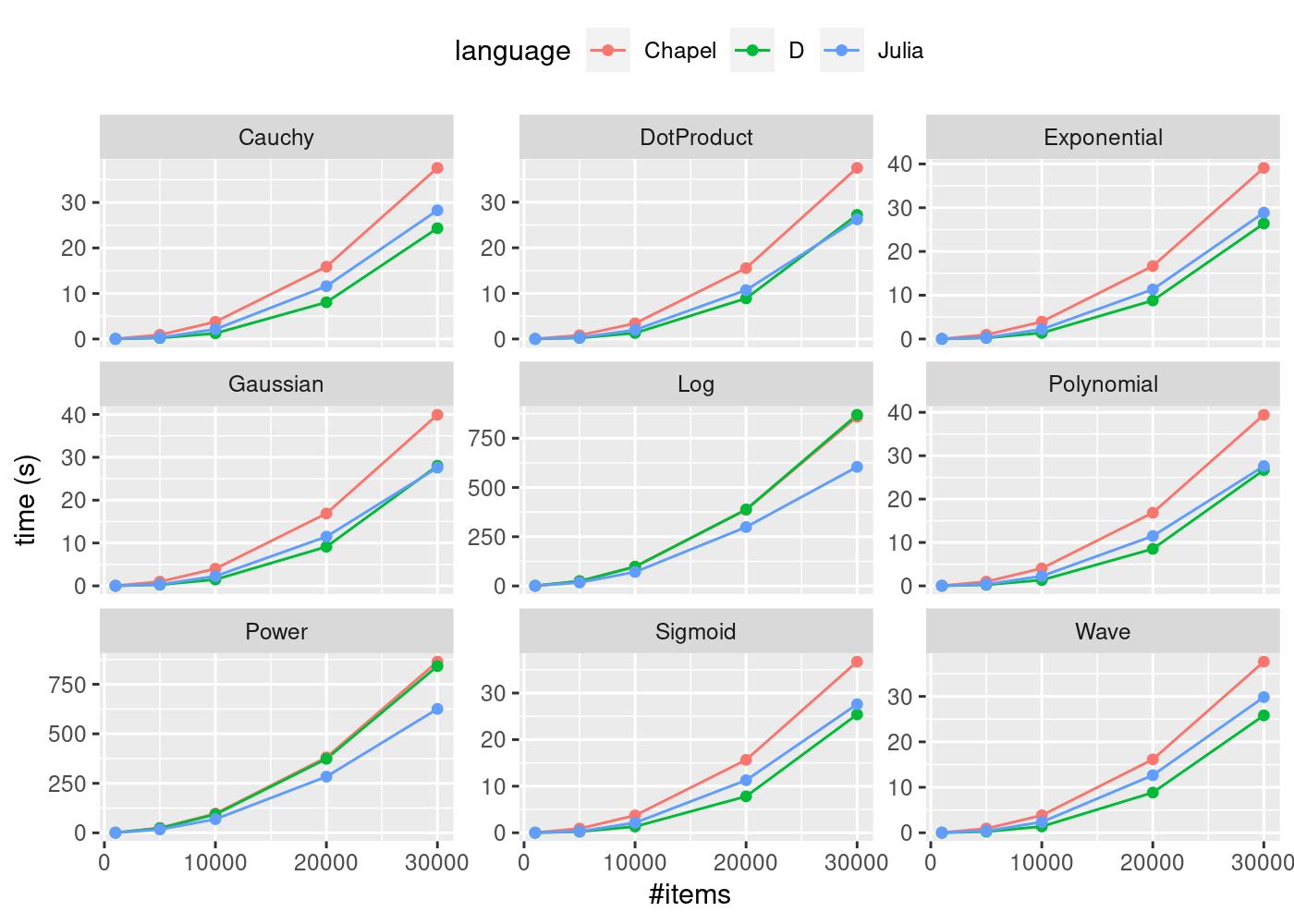
A Look at Chapel, D, and Julia Using Kernel Matrix Calculations

Introduction

It seems each time you turn around there is a new programming language aimed at solving some specific problem set. Increased proliferation of programming languages and data are deeply connected in a fundamental way, and increasing demand for “data science” computing is a related phenomenon. In the field of scientific computing, Chapel, D, and Julia are highly relevant programming languages. They arise from different needs and are aimed at different problem sets: Chapel focuses on data parallelism on single multi-core machines and large clusters; D was initially developed as a more productive and safer alternative to C++; Julia was developed for technical and scientific computing and aimed at getting the best of both worlds—the high performance and safety of static programming languages and the flexibility of dynamic programming languages. However, they all emphasize performance as a feature. In this article, we look at how their performance varies over kernel matrix calculations and present approaches to performance optimization and other usability features of the languages.

Kernel matrix calculations form the basis of kernel methods in machine learning applications. They scale rather poorly—O(m n^2), where n is the number of items and m is the number of elements in each item. In our exercsie, m will be constant and we will be looking at execution time in each implementation as n increases. Here m = 784 and n = 1k, 5k, 10k, 20k, 30k, each calculation is run three times and an average is taken. We disallow any use of BLAS and only allow use of packages or modules from the standard library of each language, though in the case of D the benchmark is compared with calculations using Mir, a multidimensional array package, to make sure that my matrix implementation reflects the true performance of D. The details for the calculation of the kernel matrix and kernel functions are given here.

While preparing the code for this article, the Chapel, D, and Julia communities were very helpful and patient with all inquiries, so they are acknowledged here.

In terms of bias, going in I was much more familiar with D and Julia than I was with Chapel. However, getting the best performance from each language required a lot of interaction with each programming community, and I have done my best to be aware of my biases and correct for them where necessary.

Language Benchmarks for Kernel Matrix Calculation

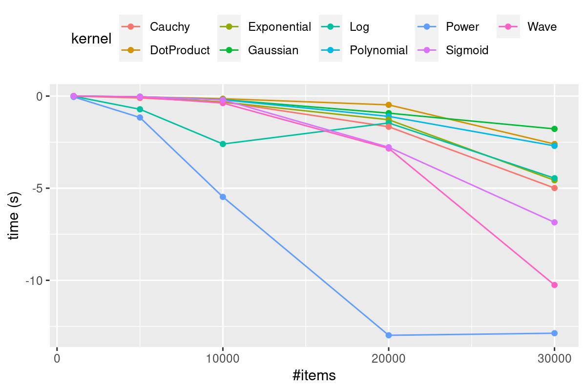
The above chart (generated using R’s ggplot2 using a script) shows the performance benchmark time taken against the number of items n for Chapel, D, and Julia, for nine kernels. D performs best in five of the nine kernels, Julia performs best in two of the nine kernels, and in two of the kernels (Dot and Gaussian) the picture is mixed. Chapel was the slowest for all of the kernel functions examined.

It is worth noting that the mathematics functions used in D were pulled from C’s math API made available in D through its core.stdc.math module because the mathematical functions in D’s standard library std.math can be quite slow. The math functions used are given here. By way of comparison, consider the mathdemo.d script comparing the imported C log function D’s log function from std.math:

$ ldc2 -O --boundscheck=off --ffast-math --mcpu=native --boundscheck=off mathdemo.d && ./mathdemo
Time taken for c log: 0.324789 seconds.
Time taken for d log: 2.30737 seconds.

The Matrix object used in the D benchmark was implemented specifically because the use of modules outside standard language libraries was disallowed. To make sure that this implementation is competitive, i.e., it does not unfairly represent D’s performance, it is compared to Mir’s ndslice library written in D. The chart below shows matrix implementation times minus ndslice times; negative means that ndslice is slower, indicating that the implementation used here does not negatively represent D’s performance.

Environment

The code was run on a computer with an Ubuntu 20.04 OS, 32 GB memory, and an Intel® Core™ i9–8950HK CPU @ 2.90GHz with 6 cores and 12 threads.

$ julia --version
julia version 1.4.1
$ dmd --version
DMD64 D Compiler v2.090.1
ldc2 --version
LDC - the LLVM D compiler (1.18.0):
  based on DMD v2.088.1 and LLVM 9.0.0
$ chpl --version
chpl version 1.22.0

Compilation

Chapel:

chpl script.chpl kernelmatrix.chpl --fast && ./script

D:

ldc2 script.d kernelmatrix.d arrays.d -O5 --boundscheck=off --ffast-math -mcpu=native && ./script

Julia (no compilation required but can be run from the command line):

julia script.jl

Implementations

Efforts were made to avoid non-standard libraries while implementing these kernel functions. The reasons for this are:

  • To make it easy for the reader after installing the language to copy and run the code. Having to install external libraries can be a bit of a “faff”.
  • Packages outside standard libraries can go extinct, so avoiding external libraries keeps the article and code relevant.
  • It’s completely transparent and shows how each language works.

Chapel

Chapel uses a forall loop to parallelize over threads. Also, C pointers to each item are used rather than the default array notation, and guided iteration over indices is used:

proc calculateKernelMatrix(K, data: [?D] ?T)
{
  var n = D.dim(0).last;
  var p = D.dim(1).last;
  var E: domain(2) = {D.dim(0), D.dim(0)};
  var mat: [E] T;
  var rowPointers: [1..n] c_ptr(T) =
    forall i in 1..n do c_ptrTo(data[i, 1]);

  forall j in guided(1..n by -1) {
    for i in j..n {
      mat[i, j] = K.kernel(rowPointers[i], rowPointers[j], p);
      mat[j, i] = mat[i, j];
    }
  }
  return mat;
}

Chapel code was the most difficult to optimize for performance and required the highest number of code changes.

D

D uses a taskPool of threads from its std.parallel package to parallelize code. The D code underwent the fewest number of changes for performance optimization—a lot of the performance benefits came from the specific compiler used and the flags selected (discussed later). My implementation of a Matrix allows columns to be selected by reference via refColumnSelect.

auto calculateKernelMatrix(alias K, T)(K!(T) kernel, Matrix!(T) data)
{
  long n = data.ncol;
  auto mat = Matrix!(T)(n, n);

  foreach(j; taskPool.parallel(iota(n)))
  {
    auto arrj = data.refColumnSelect(j).array;
    foreach(long i; j..n)
    {
      mat[i, j] = kernel(data.refColumnSelect(i).array, arrj);
      mat[j, i] = mat[i, j];
    }
  }
  return mat;
}

Julia

The Julia code uses the @threads macro for parallelising the code and @views macro for referencing arrays. One confusing thing about Julia’s arrays is their reference status. Sometimes, as in this case, arrays will behave like value objects and they have to be referenced by using the @views macro, otherwise they generate copies. At other times they behave like reference objects, for example, when passing them into a function. It can be a little tricky dealing with this because you don’t always know what set of operations will generate a copy, but where this occurs @views provides a good solution.

The Symmetric type saves the small bit of extra work needed for allocating to both sides of the matrix.

function calculateKernelMatrix(Kernel::K, data::Array{T}) where {K <: AbstractKernel,T <: AbstractFloat}
  n = size(data)[2]
  mat = zeros(T, n, n)
  @threads for j in 1:n
      @views for i in j:n
          mat[i,j] = kernel(Kernel, data[:, i], data[:, j])
      end
  end
  return Symmetric(mat, :L)
end

The @bounds and @simd macros in the kernel functions were used to turn bounds checking off and apply SIMD optimization to the calculations:

struct DotProduct <: AbstractKernel end
@inline function kernel(K::DotProduct, x::AbstractArray{T, N}, y::AbstractArray{T, N}) where {T,N}
  ret = zero(T)
  m = length(x)
  @inbounds @simd for k in 1:m
      ret += x[k] * y[k]
  end
  return ret
end

These optimizations are quite visible but very easy to apply.

Memory Usage

The total time for each benchmark and the total memory used was captured using the /usr/bin/time -v command. The output for each of the languages is given below.

Chapel took the longest total time but consumed the least amount of memory (nearly 6GB RAM peak memory):

Command being timed: "./script"
	User time (seconds): 113190.32
	System time (seconds): 6.57
	Percent of CPU this job got: 1196%
	Elapsed (wall clock) time (h:mm:ss or m:ss): 2:37:39
	Average shared text size (kbytes): 0
	Average unshared data size (kbytes): 0
	Average stack size (kbytes): 0
	Average total size (kbytes): 0
	Maximum resident set size (kbytes): 5761116
	Average resident set size (kbytes): 0
	Major (requiring I/O) page faults: 0
	Minor (reclaiming a frame) page faults: 1439306
	Voluntary context switches: 653
	Involuntary context switches: 1374820
	Swaps: 0
	File system inputs: 0
	File system outputs: 8
	Socket messages sent: 0
	Socket messages received: 0
	Signals delivered: 0
	Page size (bytes): 4096
	Exit status: 0

D consumed the highest amount of memory (around 20GB RAM peak memory) but took less total time than Chapel to execute:

Command being timed: "./script"
	User time (seconds): 106065.71
	System time (seconds): 58.56
	Percent of CPU this job got: 1191%
	Elapsed (wall clock) time (h:mm:ss or m:ss): 2:28:29
	Average shared text size (kbytes): 0
	Average unshared data size (kbytes): 0
	Average stack size (kbytes): 0
	Average total size (kbytes): 0
	Maximum resident set size (kbytes): 20578840
	Average resident set size (kbytes): 0
	Major (requiring I/O) page faults: 0
	Minor (reclaiming a frame) page faults: 18249033
	Voluntary context switches: 3833
	Involuntary context switches: 1782832
	Swaps: 0
	File system inputs: 0
	File system outputs: 8
	Socket messages sent: 0
	Socket messages received: 0
	Signals delivered: 0
	Page size (bytes): 4096
	Exit status: 0

Julia consumed a moderate amount of memory (around 7.5 GB peak memory) but ran the quickest—probably because its random number generator is the fastest:

Command being timed: "julia script.jl"
	User time (seconds): 49794.85
	System time (seconds): 30.58
	Percent of CPU this job got: 726%
	Elapsed (wall clock) time (h:mm:ss or m:ss): 1:54:18
	Average shared text size (kbytes): 0
	Average unshared data size (kbytes): 0
	Average stack size (kbytes): 0
	Average total size (kbytes): 0
	Maximum resident set size (kbytes): 7496184
	Average resident set size (kbytes): 0
	Major (requiring I/O) page faults: 794
	Minor (reclaiming a frame) page faults: 38019472
	Voluntary context switches: 2629
	Involuntary context switches: 523063
	Swaps: 0
	File system inputs: 368360
	File system outputs: 8
	Socket messages sent: 0
	Socket messages received: 0
	Signals delivered: 0
	Page size (bytes): 4096
	Exit status: 0

Performance optimization

The process of performance optimization in all three languages was very different, and all three communities were very helpful in the process. But there were some common themes.

  • Static dispatching of kernel functions instead of using polymorphism. This means that when passing the kernel function, use parametric (static compile time) polymorphism rather than runtime (dynamic) polymorphism where dispatch with virtual functions carries a performance penalty.
  • Using views/references rather than copying data over multiple threads makes a big difference.
  • Parallelising the calculations makes a huge difference.
  • Knowing if your array is row/column major and using that in your calculation makes a huge difference.
  • Bounds checks and compiler optimizations make a tremendous difference, especially in Chapel and D.
  • Enabling SIMD in D and Julia made a contribution to the performance. In D this was done using the -mcpu=native flag, and in Julia this was done using the @simd macro.

In terms of language-specific issues, getting to performant code in Chapel was the most challenging, and the Chapel code changed the most from easy-to-read array operations to using pointers and guided iterations. But on the compiler side it was relatively easy to add --fast and get a large performance boost.

The D code changed very little, and most of the performance was gained by the choice of compiler and its optimization flags. D’s LDC compiler is rich in terms of options for performance optimization. It has 8 -O optimization levels, but some are repetitions of others. For instance, -O, -O3, and -O5 are identical, and there are myriad other flags that affect performance in various ways. In this case the flags used were -O5 --boundscheck=off –ffast-math, representing aggressive compiler optimizations, bounds checking, and LLVM’s fast-math, and -mcpu=native to enable CPU vectorization instructions.

In Julia the macro changes discussed previously markedly improved the performance, but they were not too intrusive. I tried changing the optimization -O level, but this did not improve performance.

Quality of life

This section examines the relative pros and cons around the convenience and ease of use of each language. People underestimate the effort it takes to use a language day-to-day; the support and infrastructure required is significant, so it is worth comparing various facets of each language. Readers seeking to avoid the TLDR should scroll to the end of this section for the table comparing the language features discussed here. Every effort has been made to be as objective as possible, but comparing programming languages is difficult, bias prone, and contentious, so read this section with that in mind. Some elements looked at, such as arrays, are from the “data science”/technical/scientific computing point of view, and others are more general.

Interactivity

Programmers want a fast code/compile/result loop during development to quickly observe results and outputs in order to make progress or necessary changes. Julia’s interpreter is hands down the best for this and offers a smooth and feature-rich development experience, and D comes a close second. This code/compile/result loop in compilers can be slow even when compiling small code volumes. D has three compilers, the standard DMD compiler, the LLVM-based LDC compiler, and the GCC-based GDC. In this development process, the DMD and LDC compilers were used. DMD has very fast compilation times which is great for development. The LDC compiler is great at creating fast code. Chapel’s compiler is very slow in comparison. To give an example, running Linux’s time command on DMD vs Chapel’s compiler for the kernel matrix code with no optimizations gives us for D:

real	0m0.545s
user	0m0.447s
sys	0m0.101s

Compared with Chapel:

real	0m5.980s
user	0m5.787s
sys	0m0.206s

That’s a large actual and psychological difference, it can make programmers reluctant to check their work and delay the development loop if they have to wait for outputs, especially when source code increases in volume and compilation times become significant.

It is worth mentioning, however, that when developing packages in Julia, compilation times can be very long, and users have noticed that when they load some packages ,compilation times can stretch. So the experience of the development loop in Julia could vary, but in this specific case the process was seamless.

Documentation and examples

One way of comparing documentation in the different languages is to compare them all with Python’s official documentation, which is the gold standard for programming languages. It combines examples with formal definitions and tutorials in a seamless and user-friendly way. Since many programmers are familiar with the Python documentation, this approach gives an idea of how they compare.

Julia’s documentation is the closest to Python’s documentation quality and gives the user a very smooth, detailed, and relatively painless transition into the language. It also has a rich ecosystem of blogs, and topics on many aspects of the language are easy to come by. D’s official documentation is not as good and can be challenging and frustrating, however there is a very good free book “Programming in D” which is a great introduction to the language, but no single book can cover a programming language and there are not many sources for advanced topics. Chapel’s documentation is quite good for getting things done, though examples vary in presence and quality. Often, the programmer needs a lot of knowledge to look in the right place. A good topic for comparison is file I/O libraries in Chapel, D, and Julia. Chapel’s I/O library has too few examples but is relatively clear and straightforward; D’s I/O is kind of spread across a few modules, and documentation is more difficult to follow; Julia’s I/O documentation has lots of examples and is clear and easy to follow.

Perhaps one factor affecting Chapel’s adoption is lack of example—since its arrays have a non-standard interface, the user has to work hard to become familiar with them. Whereas even though D’s documentation may not be as good in places, the language has many similarities to C and C++, so it gets away with more sparse documentation.

Multi-dimensional Array support

“Arrays” here does not refer to native C and C++ style arrays available in D, but mathematical arrays. Julia and Chapel ship with array support and D does not, but it has the Mir library which has multidimensional arrays (ndslice). In the implementation of kernel matrix, I wrote my own matrix object in D, which is not difficult if you understand the principle, but it’s not something a user wants to do. However, D has a linear algebra library called Lubeck which has impressive performance characteristics and interfaces with all the usual BLAS implementations. Julia’s arrays are by far the easiest and most familiar. Chapel’s arrays are more difficult to get started with than Julia’s but are designed to be run on single-core, multi-core, and computer clusters using the same or very similar code, which is a good unique selling point.

Language power

Since Julia is a dynamic programming language, some might say, “well Julia is a dynamic language which is far more permissive than static programming languages, therefore the debate is over”, but it’s more complicated than that. There is power in static type systems. Julia has a type system similar in nature to type systems from static languages, so you can write code as if you were using a static language, but you can do things reserved only for dynamic languages. It has a highly developed generic and meta-programming syntax and powerful macros. It also has a highly flexible object system and multiple dispatch. This mix of features is what makes Julia the most powerful language of the three.

D was intended to be a replacement for C++ and takes very much after C++ (and also borrows from Java), but makes template programming and compile-time evaluation much more user-friendly than in C++. It is a single dispatch language (though multi-methods are available in a package). Instead of macros, D has string and template “mixins” which serve a similar purpose.

Chapel has generic programming support and nascent support for single dispatch OOP, no macro support, and is not yet as mature as D or Julia in these terms.

Concurrency & Parallel Programming

Nowadays, new languages tout support for concurrency and its popular subset, parallelism, but the details vary a lot between languages. Parallelism is more relevant in this example and all three languages deliver. Writing parallel for loops is straightforward in all three languages.

Chapel’s concurrency model has much more emphasis on data parallelism but has tools for task parallelism and ships with support for cluster-based concurrency.

Julia has good support for both concurrency and parallelism.

D has industry strength support for parallelism and concurrency, though its support for threading is much less well documented with examples.

Standard Library

How good is the standard library of all three languages in general? What range of tasks do they allow users to easily tend to? It’s a tough question because library quality and documentation factor in. All three languages have very good standard libraries. D has the most comprehensive standard library, but Julia is a great second, then Chapel, but things are never that simple. For example, a user seeking to write binary I/O may find Julia the easiest to start with; it has the most straightforward, clear interface and documentation, followed by Chapel, and then D. Though in my implementation of an IDX file reader, D’s I/O was the fastest, but then Julia code was easy to write for cases unavailable in the other two languages.

Package Managers & Package Ecosystems

In terms of documentation, usage, and features, D’s Dub package manager is the most comprehensive. D also has a rich package ecosystem in the Dub website, Julia’s package manager runs tightly integrated with GitHub and is a good package system with good documentation. Chapel has a package manager but does not have a highly developed package ecosystem.

C Integration

C interop is easy in all three languages; Chapel has good documentation but is not as well popularised as the others. D’s documentation is better and Julia’s documentation is the most comprehensive. Oddly enough though, none of the languages’ documentation show the commands required to compile your own C code and integrate it with the language, which is an oversight especially when it comes to novices. It is, however, easy to search for and find examples for the compilation process in D and Julia.

Community

All three languages have convenient places where users can ask questions. For Chapel, the easiest place is Gitter, for Julia it’s Discourse (though there is a Julia Gitter), and for D it’s the official website forum. The Julia community is the most active, followed by D, and then Chapel. I’ve found that you’ll get good responses from all three communities, but you’ll probably get quicker answers from the D and Julia communities.

Chapel D Julia
Compilation/Interactivty Slow Fast Best
Documentation & Examples Detailed Patchy Best
Multi-dimensional Arrays Yes Native Only
(library support)
Yes
Language Power Good Great Best
Concurrency & Parallelism Great Great Good
Standard Library Good Great Great
Package Manager & Ecosystem Nascent Best Great
C Integration Great Great Great
Community Small Vibrant Largest

Table for quality of life features in Chapel, D & Julia

Summary

If you are a novice programmer writing numerical algorithms and doing calculations based in scientific computing and want a fast language that’s easy to use, Julia is your best bet. If you are an experienced programmer working in the same space, Julia is still a great option. If you specifically want a more conventional, “industrial strength”, statically compiled, high-performance language with all the “bells and whistles”, but want something more productive, safer, and less painful than C++, then D is your best bet. You can write “anything” in D and get great performance from its compilers. If you need to get array calculations happening on clusters, then Chapel is probably the easiest place to go.

In terms of raw performance on this task, D was the winner, clearly performing better in 5 out of the 9 kernels benchmarked. This exercise reveals that Julia’s label as a high-performance language is more than just hype—it has held it’s own against highly competitive languages. It was harder than expected to get competitive performance from Chapel—it took a lot of investigation from the Chapel team to come up with the current solution. However, as the Chapel language matures we could see further improvement.

Lomuto’s Comeback

The Continental Club in Austin, Texas, USA
Sunday, January 5, 1987

“Thank you for your kind invitation, Mr. Lomuto. I will soon return to England so this is quite timely.”

“And thanks for agreeing to meeting me, Mister… Sir… Charles… A.R… Hoare. It’s a great honor. I don’t even know how to address you. Were you knighted?”

“Call me Tony, and if it’s not too much imposition please allow me to call you Nico.”

On the surface, a banal scene—two men enjoying a whiskey. However, a closer look revealed a number of intriguing details. For starters, a tension you could cut with a knife.

Dressed in a perfectly tailored four-piece suit worn with the nonchalance only an Englishman could pull off, Tony Hoare was as British as a cup of tea. His resigned grimaces as he was sipping from his glass spoke volumes about his opinion of Bourbon versus Scotch. On the other side of the small table, Nico Lomuto couldn’t have been more different: a casually dressed coder enjoying his whiskey with Coca-Cola (a matter so outrageous that Tony had decided early on to studiously pretend not to notice, as he would when confronted with ripe body odor or an offensive tattoo), in a sort of relaxed awe at the sight of the Computer Science giant he had just met.

“Listen, Tony,” Nico said as the chit chat petered off, “about that partitioning algorithm. I never meant to publish or—”

“Oh? Yes, yes, the partitioning algorithm.” Tony’s eyebrows rose with feigned surprise, as if it had escaped his mind that every paper and book on quicksort in the past five years mentioned their names together. It was obviously the one thing connecting the two men and the motivation of the meeting, but Tony, the perfect gentleman, could talk about the weather for hours with a pink elephant in the room if his conversation partner didn’t bring it up.

“Yeah, that partitioning algorithm that keeps on getting mentioned together with yours,” Nico continued. “I’m not much of an algorithms theorist. I’m working on Ada, and this entire thing about my partition scheme is a distraction. The bothersome part about it”—Nico was speaking in the forthcoming tone of a man with nothing to hide—”is that it’s not even a better algorithm. My partitioning scheme will always do the same number of comparisons and at least as many swaps as yours. In the worst case, mine does n additional swaps—n! I can’t understand why they keep on mentioning the blessed thing. It’s out of my hands now. I can’t tell them what algorithms to teach and publish. It’s like bubblesort. Whenever anyone mentions quicksort, there’s some chowderhead—or should I say bubblehead—in the audience going, yes, I also heard of the bubblesort algorithm. Makes my blood curdle.”

Nico sighed. Tony nodded. Mutual values. Rapport filled the air in between as suddenly, quietly, and pleasantly as the smell of cookies out of the oven. A few seconds went by. Jack and Coke sip. On the other side of the table, Bourbon sip, resigned grimace.

Tony spoke with the carefully chosen words of a scientist who wants to leave no hypothesis unexplored. “I understand, Nico. Yet please consider the following. Your algorithm is simple and regular, moves in only one direction, and does at most one swap per step. That may be appropriate for some future machines that…”

“No matter the machine, more swaps can’t be better than fewer swaps. It’s common sense,” Nico said, peremptorily.

“I would not be so sure. Computers do not have common sense. Computers are surprising. It stands to reason they’ll continue to be. Well, how about we enjoy this evening. Nothing like a good conversation in a quiet club.”

“Yeah. Cheers. This is a fun place. I hear they’ll have live country music soon.”

“Charming.” Somewhat to his own surprise, Tony mustered a polite smile.

Chestnut Hill, Massachusetts, USA
Present Day

I’ve carried an unconfessed addiction to the sorting problem for many years. Wasn’t that difficult to hide—to a good extent, an obsessive inclination to studying sorting is a socially tolerated déformation professionnelle; no doubt many a programmer has spent a few late nights trying yet another sorting idea that’s going to be so much better than the others. So nobody raised an eyebrow when I wrote about sorting all the way back in 2002 (ever heard about “fit pivot?” Of course you didn’t). There was no intervention organized when I wrote D’s std.sort, which turned out to be sometimes quadratic (and has been thankfully fixed since). No scorn even when I wrote an academic paper on the selection problem (sort’s cousin) as an unaffiliated outsider, which even the conference organizers said was quite a trick. And no public outrage when I spoke about sorting at CppCon 2019. Coders understand.

So, I manage. You know what they say—one day at a time. Yet I did feel a tinge of excitement when I saw the title of a recent paper: “Branch Mispredictions Don’t Affect Mergesort.” Such an intriguing title. To start with, are branch mispredictions expected to affect mergesort? I don’t have much of an idea, mainly because everybody and their cat is using quicksort, not mergesort, so the latter hasn’t really been at the center of my focus. But hey, I don’t even need to worry about it because the title resolutely asserts that that problem I didn’t know I was supposed to worry about, I don’t need to worry about after all. So in a way the title cancels itself out. Yet I did read the paper (and recommend you do the same) and among many interesting insights, there was one that caught my attention: Lomuto’s partitioning scheme was discussed as a serious contender (against the universally-used Hoare partition) from an efficiency perspective. Efficiency!

It turns out modern computing architecture does, sometimes, violate common sense.

To Partition, Perchance to Sort

Let’s first recap the two partitioning schemes. Given an array and a pivot element, to partition the array means to arrange elements of the array such that all elements smaller than or equal to the pivot are on the left, and elements greater than or equal to the pivot are on the right. The final position of the pivot would be at the border. (If there are several equivalent pivot values that final pivot position may vary, with important practical consequences; for this discussion, however, we can assume that all array values are distinct.)

Lomuto’s partitioning scheme walks the array left to right maintaining a “read” position and a “write” position, both initially at 0. For each element read, if the value seen by the “read head” is greater than the pivot, it gets skipped (with the read head moving to the next position). Otherwise, the value at the read head is swapped with that at the write head, and both heads advance by one position. When the read head is done, the position of the write head defines the partition. Refer to the nice animation below (from Wikipedia user Mastremo, used unmodified under the CC-BY-SA 3.0 license).

The problem with Lomuto’s partition is that it may do unnecessary swaps. Consider the extreme case of an array with only the leftmost element greater than the pivot. That element will be awkwardly moved to the right one position per iteration step, in a manner not unlike, um, bubblesort.

Hoare’s partitioning scheme elegantly solves that issue by iterating concomitantly from both ends of the array with two “read/write heads”. They skip elements that are already appropriately placed (less than the pivot on the left, greater than the pivot on the right), and swap only one smaller element from the left with one greater element from the right. When the two heads meet, the array is partitioned around the meet point. The extreme case described above is handled with a single swap. Most contemporary implementations of quicksort use Hoare partition, for obvious reasons: it does as many comparisons as the Lomuto partition and fewer swaps.

Given that Hoare partition clearly does less work than Lomuto partition, the question would be why ever teach or use the latter at all. Alexander Stepanov, the creator of the STL, authored a great discussion about partitioning and makes a genericity argument: Lomuto partition only needs forward iterators, whereas Hoare partition requires bidirectional iterators. That’s a valuable insight, albeit of limited practical utility: yes, you could use Lomuto’s partition on singly-linked lists, but most of the time you partition for quicksort’s sake, and you don’t want to quicksort singly-linked lists; mergesort would be the algorithm of choice.

Yet a very practical—and very surprising—argument does exist, and is the punchline of this article: implemented in a branch-free manner, Lomuto partition is a lot faster than Hoare partition on random data. Given that quicksort spends most of its time partitioning, it follows that we are looking at a hefty improvement of quicksort (yes, I am talking about industrial strength implementations for C++ and D) by replacing its partitioning algorithm with one that literally does more work.

You read that right.

Time to Spin Some Code

To see how the cookie crumbles, let’s take a look at a careful implementation of Hoare partition. To eliminate all extraneous details, the code in this article is written for long as the element type and uses raw pointers. It compiles and runs the same with a C++ or D compiler. This article will carry along implementations of all routines in both languages because much research literature measures algorithm performance using C++’s std::sort as an important baseline.

/**
Partition using the minimum of the first and last element as pivot.
Returns: a pointer to the final position of the pivot.
*/
long* hoare_partition(long* first, long* last) {
    assert(first <= last);
    if (last - first < 2)
        return first; // nothing interesting to do
    --last;
    if (*first > *last)
        swap(*first, *last);
    auto pivot_pos = first;
    auto pivot = *pivot_pos;
    for (;;) {
        ++first;
        auto f = *first;
        while (f < pivot)
            f = *++first;
        auto l = *last;
        while (pivot < l)
            l = *--last;
        if (first >= last)
            break;
        *first = l;
        *last = f;
        --last;
    }
    --first;
    swap(*first, *pivot_pos);
    return first;
}

(You may find the choice of pivot a bit odd, but not to worry: usually it’s a more sophisticated scheme—such as median-of-3—but what’s important to the core loop is that the pivot is not the largest element of the array. That allows the core loop to omit a number of limit conditions without running off array bounds.)

There are a lot of good things to say about the efficiency of this implementation (which you’re likely to find, with minor details changed, in implementations of the C++ or D standard library). You could tell the code above was written by people who live trim lives. People who keep their nails clean, show up when they say they’ll show up, and call Mom regularly. They do a wushu routine every morning and don’t let computer cycles go to waste. That code has no slack in it. The generated Intel assembly is remarkably tight and virtually identical for C++ and D. It only varies across backends, with LLVM at a slight code size advantage (see clang and ldc) over gcc (see g++ and gdc).

The initial implementation of Lomuto’s partition shown below works well for exposition, but is sloppy from an efficiency perspective:

/**
Choose the pivot as the first element, then partition.
Returns: a pointer to the final position of the pivot. 
*/
long* lomuto_partition_naive(long* first, long* last) {
    assert(first <= last);
    if (last - first < 2)
        return first; // nothing interesting to do
    auto pivot_pos = first;
    auto pivot = *first;
    ++first;
    for (auto read = first; read < last; ++read) {
        if (*read < pivot) {
            swap(*read, *first);
            ++first;
        }
    }
    --first;
    swap(*first, *pivot_pos);
    return first;
}

For starters, the code above will do a lot of silly no-op swaps (array element with itself) if a bunch of elements on the left of the array are greater than the pivot. All that time first==write, so swapping *first with *write is unnecessary and wasteful. Let’s fix that with a pre-processing loop that skips the uninteresting initial portion:

/**
Partition using the minimum of the first and last element as pivot. 
Returns: a pointer to the final position of the pivot.
*/
long* lomuto_partition(long* first, long* last) {
    assert(first <= last);
    if (last - first < 2)
        return first; // nothing interesting to do
    --last;
    if (*first > *last)
        swap(*first, *last);
    auto pivot_pos = first;
    auto pivot = *first;
    // Prelude: position first (the write head) on the first element
    // larger than the pivot.
    do {
        ++first;
    } while (*first < pivot);
    assert(first <= last);
    // Main course.
    for (auto read = first + 1; read < last; ++read) {
        auto x = *read;
        if (x < pivot) {
            *read = *first;
            *first = x;
            ++first;
        }
    }
    // Put the pivot where it belongs.
    assert(*first >= pivot);
    --first;
    *pivot_pos = *first;
    *first = pivot;
    return first;
}

The function now chooses the pivot as the smallest of first and last element, just like hoare_partition. I also made another small change—instead of using the swap routine, let’s use explicit assignments. The optimizer takes care of that automatically (enregistering plus register allocation for the win), but expressing it in source helps us see the relatively expensive array reads and array writes. Now for the interesting part. Let’s focus on the core loop:

for (auto read = first + 1; read < last; ++read) {
    auto x = *read;
    if (x < pivot) {
        *read = *first;
        *first = x;
        ++first;
    }
}

Let’s think statistics. There are two conditionals in this loop: read < last and x < pivot. How predictable are they? Well, the first one is eminently predictable—you can reliably predict it will always be true, and you’ll only be wrong once no matter how large the array is. Compiler writers and hardware designers know this, and design the fastest path under the assumption loops will continue. (Gift idea for your Intel engineer friend: a doormat that reads “The Backward Branch Is Always Taken.”) The CPU will speculatively start executing the next iteration of the loop even before having decided whether the loop should continue. That work will be thrown away only once, at the end of the loop. That’s the magic of speculative execution.

Things are quite a bit less pleasant with the second test, x < pivot. If you assume random data and a randomly-chosen pivot, it could go either way with equal probability. That means speculative execution is not effective at all, which is very bad for efficiency. How bad? In a deeply pipelined architecture (as all are today), failed speculation means the work done by several pipeline stages needs to be thrown away, which in turn propagates a bubble of uselessness through the pipeline (think air bubbles in a garden hose). If these bubbles occur too frequently, the loop produces results at only a fraction of the attainable bandwidth. As the measurements section will show, that one wasted speculation takes away about 30% of the potential speed.

How to improve on this problem? Here’s an idea: instead of making decisions that control the flow of execution, we write the code in a straight-line manner and we incorporate the decisions as integers that guide the data flow by means of carefully chosen array indexing. Be prepared—this will force us to do silly things. For example, instead of doing two conditional writes per iteration, we’ll do exactly two writes per iteration no matter what. If the writes were not needed, we’ll overwrite words in memory with their own value. (Did I mention “silly things”?) To prepare the code for all that, let’s rewrite it as follows:

for (auto read = first + 1; read < last; ++read) {
    auto x = *read;
    if (x < pivot) {
        *read = *first;
        *first = x;
        first += 1; 
    } else {
        *read = x;
        *first = *first;
        first += 0; 
    }
}

Now the two branches of the loop are almost identical save for the data. The code is still correct (albeit odd) because on the else branch it needlessly writes *read over itself and *first over itself. How do we now unify the two branches? Doing so in an efficient manner takes a bit of pondering and experimentation. Conditionally incrementing first is easy because we can always write first += x < pivot. Piece of cake. The two memory writes are more difficult, but the basic idea is to take the difference between pointers and use indexing. Here’s the code. Take a minute to think it over:

for (; read < last; ++read) {
    auto x = *read;
    auto smaller = -int(x < pivot);
    auto delta = smaller & (read - first);
    first[delta] = *first;
    read[-delta] = x;
    first -= smaller;
}

To paraphrase a famous Latin aphorism, explanatio longa, codex brevis est. Short is the code, long is the ‘splanation. The initialization of smaller with -int(x < pivot) looks odd but has a good reason: smaller can serve as both an integral (0 or -1) used with the usual arithmetic and also as a mask that is 0 or 0xFFFFFFFF (i.e. bits set all to 0 or all to 1) used with bitwise operations. We will use that mask to allow or obliterate another integral in the next line that computes delta. If x < pivotsmaller is all ones and delta gets initialized to read - first. Subsequently, delta is used in first[delta] and read[-delta], which really are syntactic sugar for *(first + delta) and *(read - delta), respectively. If we substitute delta in those expressions, we obtain *(first + (read - first)) and *(read - (read - first)), respectively.

The last line, first -= smaller, is trivial: if x < pivot, subtract -1 from first, which is the same as incrementing first. Otherwise, subtract 0 from first, effectively leaving first alone. Nicely done.

With x < pivot substituted to 1, the calculation done in the body of the loop becomes:

auto x = *read;
int smaller = -1;
auto delta = -1 & (read - first);
*(first + (read - first)) = *first;
*(read - (read - first)) = x;
first -= -1;

Kind of magically the two pointer expressions simplify down to *read and *first, so the two assignments effect a swap (recall that x had been just initialized with *read). Exactly what we did in the true branch of the test in the initial version!

If x < pivot is false, delta gets initialized to zero and the loop body works as follows:

auto x = *read;
int smaller = 0;
auto delta = 0 & (read - first);
*(first + 0) = *first;
*(read - 0) = x;
first -= 0;

This time things are simpler: *first gets written over itself, *read also gets written over itself, and first is left alone. The code has no effect whatsoever, which is exactly what we wanted.

Let’s now take a look at the entire function:

long* lomuto_partition_branchfree(long* first, long* last) {
    assert(first <= last);
    if (last - first < 2)
        return first; // nothing interesting to do
    --last;
    if (*first > *last)
        swap(*first, *last);
    auto pivot_pos = first;
    auto pivot = *first;
    do {
        ++first;
        assert(first <= last);
    } while (*first < pivot);
    for (auto read = first + 1; read < last; ++read) {
        auto x = *read;
        auto smaller = -int(x < pivot);
        auto delta = smaller & (read - first);
        first[delta] = *first;
        read[-delta] = x;
        first -= smaller;
    }
    assert(*first >= pivot);
    --first;
    *pivot_pos = *first;
    *first = pivot;
    return first;
}

A beaut, isn’t she? Even more beautiful is the generated code—take a look at clang/ldc and g++/gdc. Again, there is a bit of variation across backends.

Experiments and Results

All code is available at https://github.com/andralex/lomuto.

To draw a fair comparison between the two partitioning schemes, I’ve put together a quicksort implementation. This is because most often a partition would be used during quicksort. For the sake of simplification, the test implementation omits a few details present in industrial quicksort implementations, which need to worry about a variety of data shapes (partially presorted ascending or descending, with local patterns, with many duplicates, etc). Library implementations choose the pivot carefully from a sample of usually 3-9 elements, possibly with randomization, and have means to detect and avoid pathological inputs, most often by using Introsort.

In our benchmark, for simplicity, we only test against random data, and the choice of pivot is simply the minimum of first and last element. This is without loss of generality; better pivot choices and adding introspection are done the same way regardless of the partitioning method. Here, the focus is to compare the performance of Hoare vs. Lomuto vs. branch-free Lomuto.

The charts below plot the time taken by one sorting operation depending on the input size. The machine used is an Intel i7-4790 at 3600 MHz with a 256KB/1MB/8MB cache hierarchy running Ubuntu 20.04. All builds were for maximum speed (-O3, no assertions, no boundcheck for the D language). The input is a pseudorandom permutation of longs with the same seed for all languages and platforms. To eliminate noise, the minimum is taken across several epochs.

The results for the D language are shown below, including the standard library’s std.sort as a baseline.

Chart by Visualizer
Chart by Visualizer

The results for C++ are shown in the plots below. Again the standard library implementation std::sort is included as a baseline.

Chart by Visualizer
Chart by Visualizer

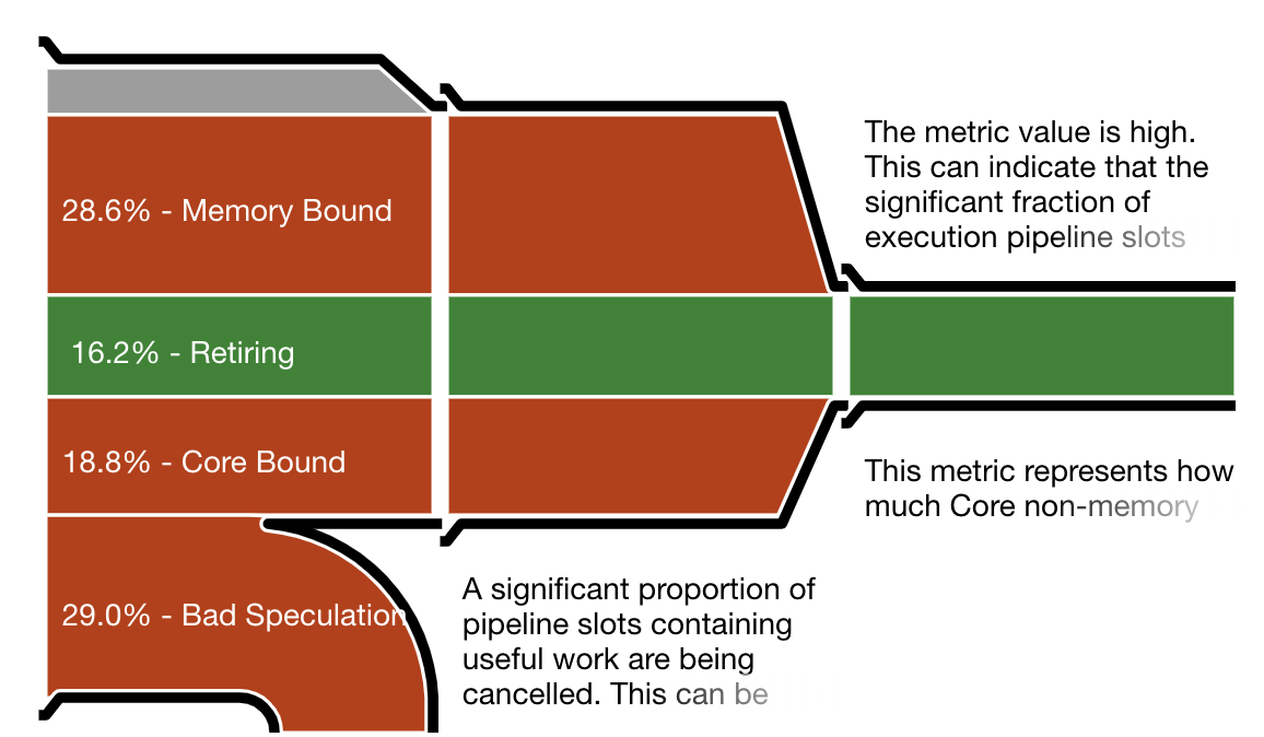
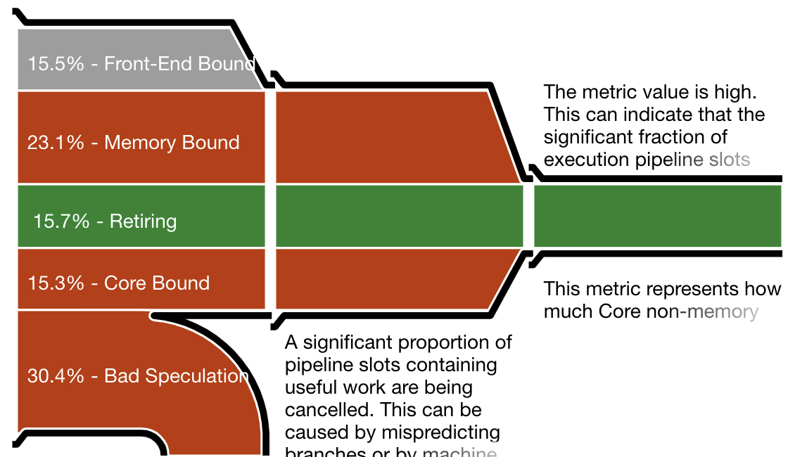
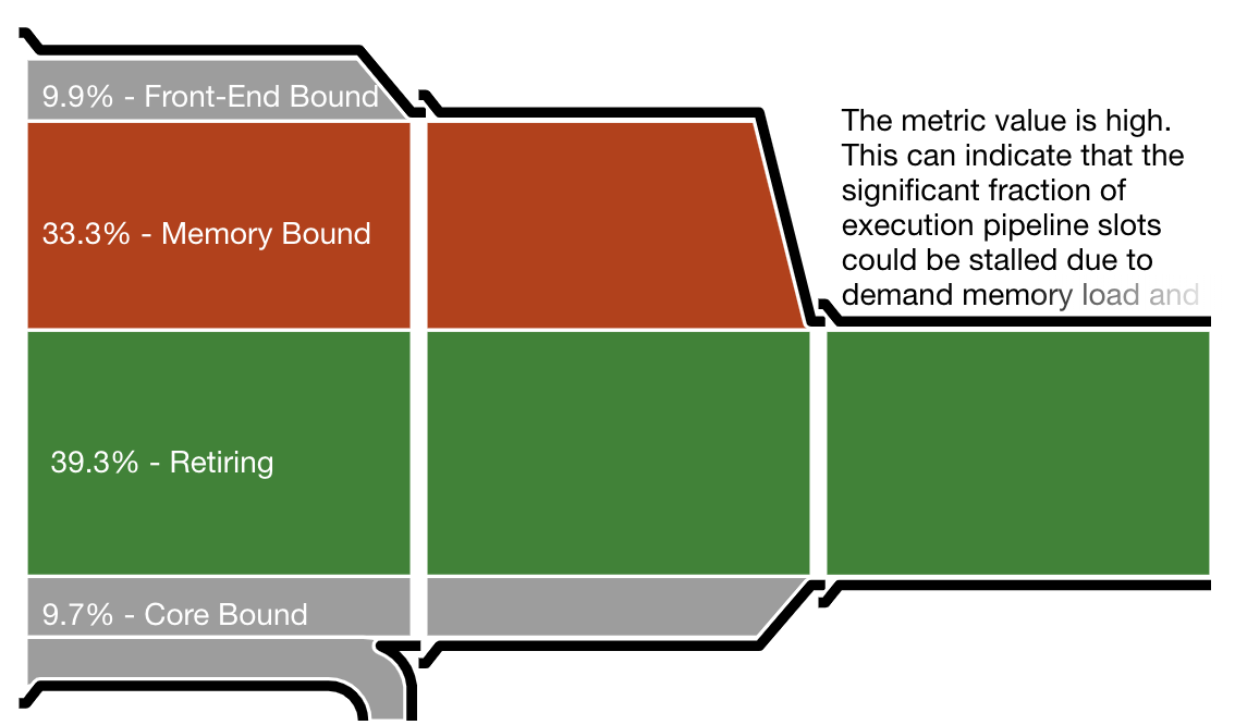
One important measurement is the CPU utilization efficiency, shown by Intel VTune as “the micropipe”, a diagram illustrating inefficiencies in resource utilization. VTune’s reports are very detailed but the micropipe gives a quick notion of where the work goes. To interpret a micropipe, think of it as a funnel. The narrower the exit (on the right), the slower the actual execution as a fraction of potential speed.

The micropipes shown below correspond to the Hoare partition, Lomuto partition (in the traditional implementation), and branch-free Lomuto partition. The first two throw away about 30% of all work as bad speculation. In contrast, the Lomuto branchless partition wastes no work on speculation, which allows it a better efficiency in spite of more memory writes.

Intel VTune pipe efficiency diagram for the Hoare partition. A large percentage of work is wasted on failed speculation.

Intel VTune pipe efficiency diagram for the traditional “branchy” Lomuto partition, featuring about as much failed speculation as the Hoare partition.

Intel VTune pipe efficiency diagram for the Lomuto branch-free partition. Virtually no work is wasted on failed speculation, leading to a much better efficiency.

Discussion

The four versions (two languages times two backends) exhibit slight variations due to differences in standard library implementations and backend versions. It is not surprising that minute variations in generated code are liable to create measurable differences in execution speed.

As expected, the “branchy” Lomuto partition compares poorly with Hoare partition, especially for large input sizes. Both are within the same league as the standard library implementation of the sort routine. Sorting using the branchless Lomuto partition, however, is the clear winner by a large margin regardless of platform, backend, and input size.

It has become increasingly clear during the past few years that algorithm analysis—and proposals for improvements derived from it—cannot be done solely with pen and paper using stylized computer architectures with simplistic cost models. The efficiency of sorting is determined by a lot more than counting the comparisons and swaps—at least, it seems, the predictability of comparisons must be taken into account. In the future, I am hopeful that better models of computation will allow researchers to rein in the complexity. For the time being, it seems, algorithm optimization remains hopelessly experimental.

For sorting in particular, Lomuto is definitely back and should be considered by industrial implementations of quicksort on architectures with speculative execution.

Acknowledgments

Many thanks are due to Amr Elmasry, Jyrki Katajainen, and Max Stenmark for an inspirational paper. I haven’t yet been able to engineer a mergesort implementation (the main result of their paper) that beats the best quicksort described here, but I’m working on it. (Sorry, Sorters Anonymous… I’m still off the wagon.) I’d like to thank to Michael Parker and the commentators at the end of this post for fixing many of my non-native-speaker-isms. (Why do they say “pretend not to notice” and “pretend to not notice”? I never remember the right one.) Of course, most of the credit is due to Nico Lomuto, who defined an algorithm that hasn’t just stood the test of time—it passed it.

Interfacing D with C: Arrays and Functions (Arrays Part 2)

Digital Mars D logo

This post is part of an ongoing series on working with both D and C in the same project. The previous post explored the differences in array declaration and initialization. This post takes the next step: declaring and calling C functions that take arrays as parameters.

Arrays and C function declarations

Using C libraries in D is extremely easy. Most of the time, things work exactly as one would expect, but as we saw in the previous article there can be subtle differences. When working with C functions that expect arrays, it’s necessary to fully understand these differences.

The most straightforward and common way of declaring a C function that accepts an array as a parameter is to to use a pointer in the parameter list. For example, this hypothetical C function:

void f0(int *arr);

In C, any array of int can be passed to this function no matter how it was declared. Given int a[], int b[3], or int *c, the function calls f0(a), f0(b), and f0(c) are all the same: a pointer to the first element of each array is passed to the function. Or using the lingo of C programmers, arrays decay to pointers

Typically, in a function like f0, the implementer will expect the array to have been terminated with a marker appropriate to the context. For example, strings in C are arrays of char that are terminated with the \0 character (we’ll look at D strings vs. C strings in a future post). This is necessary because, without that character, the implementation of f0 has no way to know which element in the array is the last one. Sometimes, a function is simply documented to expect a certain length, either in comments or in the function name, e.g., a vector3f_add(float *vec) will expect that vec points to exactly 3 elements. Another option is to require the length of the array as a separate argument:

void f1(int *arr, size_t len);

None of these approaches is foolproof. If f0 receives an array with no end marker or which is shorter than documented, or if f1 receives an array with an actual length shorter than len, then the door is open for memory corruption. D arrays take this possibility into account, making it much easier to avoid such problems. But again, even D’s safety features aren’t 100% foolproof when calling C functions from D.

There are other, less common, ways array parameters may be declared in C:

void f2(int arr[]);
void f3(int arr[9]);
void f4(int arr[static 9]);

Although these parameters are declared using C’s array syntax, they boil down to the exact same function signature as f0 because of the aforementioned pointer decay. The [9] in f3 triggers no special enforcement by the compiler; arr is still effectively a pointer to int with unknown length. The [9] serves as documentation of what the function expects, and the implementation cannot rely on the array having nine elements.

The only potential difference is in f4. The static added to the declaration tells the compiler that the function must take an array of, in this case, at least nine elements. It could have more than nine, but it can’t have fewer. That also rules out null pointers. The problem is, this isn’t necessarily enforced. Depending on which C compiler you use, if you shortchange the function and send it less than nine elements you might see warnings if they are enabled, but the compiler might not complain at all. (I haven’t tested current compilers for this article to see if any are actually reporting errors for this, or which ones provide warnings.)

The behavior of C compilers doesn’t matter from the D side. All we need be concerned with is declaring these functions appropriately so that we can call them from D such that there are no crashes or unexpected results. Because they are all effectively the same, we could declare them all in D like so:

extern(C):
void f0(int* arr);
void f1(int* arr, size_t len);
void f2(int* arr);
void f3(int* arr);
void f4(int* arr);

But just because we can do a thing doesn’t mean we should. Consider these alternative declarations of f2, f3, and f4:

extern(C):
void f2(int[] arr);
void f3(int[9] arr);
void f4(int[9] arr);

Are there any consequences of taking this approach? The answer is yes, but that doesn’t mean we should default to int* in each case. To understand why, we need first to explore the innards of D arrays.

The anatomy of a D array

The previous article showed that D makes a distinction between dynamic and static arrays:

int[] a0;
int[9] a1;

a0 is a dynamic array and a1 is a static array. Both have the properties .ptr and .length. Both may be indexed using the same syntax. But there are some key differences between them.

Dynamic arrays

Dynamic arrays are usually allocated on the heap (though that isn’t a requirement). In the above case, no memory for a0 has been allocated. It would need to be initialized with memory allocated via new or malloc, or some other allocator, or with an array literal. Because a0 is uninitialized, a0.ptr is null and a0.length is 0.

A dynamic array in D is an aggregate type that contains the two properties as members. Something like this:

struct DynamicArray {
    size_t length;
    size_t ptr;
}

In other words, a dynamic array is essentially a reference type, with the pointer/length pair serving as a handle that refers to the elements in the memory address contained in the ptr member. Every built-in D type has a .sizeof property, so if we take a0.sizeof, we’ll find it to be 8 on 32-bit systems, where size_t is a 4-byte uint, and 16 on 64-bit systems, where size_t is an 8-byte ulong. In short, it’s the size of the handle and not the cumulative size of the array elements.

Static arrays

Static arrays are generally allocated on the stack. In the declaration of a1, stack space is allocated for nine int values, all of which are initialized to int.init (which is 0) by default. Because a1 is initialized, a1.ptr points to the allocated space and a1.length is 9. Although these two properties are the same as those of the dynamic array, the implementation details differ.

A static array is a value type, with the value being all of its elements. So given the declaration of a1 above, its nine int elements indicate that a1.sizeof is 9 * int.sizeof, or 36. The .length property is a compile-time constant that never changes, and the .ptr property, though not readable at compile time, is also a constant that never changes (it’s not even an lvalue, which means it’s impossible to make it point somewhere else).

These implementation details are why we must pay attention when we cut and paste C array declarations into D source modules.

Passing D arrays to C

Let’s go back to the declaration of f2 in C and give it an implementation:

void f2(int arr[]) {
    for(int i=0; i<3; ++i)
        printf("%d\n", arr[i]);
}

A naïve declaration in D:

extern(C) void f2(int[]);

void main() {
    int[] a = [10, 20, 30];
    f2(a);
}

I say naïve because this is never the right answer. Compiling f2.c with df2.d on Windows (cl /c f2.c in the “x64 Native Tools” command prompt for Visual Studio, followed by dmd -m64 df2.d f2.obj), then running df2.exe, shows me the following output:

3
0
1970470928

There is no compiler error because the declaration of f2 is pefectly valid D. The extern(C) indicates that this function uses the cdecl calling convention. Calling conventions affect the way arguments are passed to functions and how the function’s symbol is mangled. In this case, the symbol will be either _f2 or f2 (other calling conventions, like stdcallextern(Windows) in D—have different mangling schemes). The declaration still has to be valid D. (In fact, any D function can be marked as extern(C), something which is necessary when creating a D library that will be called from other languages.)

There is also no linker error. DMD is calling out to the system linker (in this case, Microsoft’s link.exe), the same linker used by the system’s C and C++ compilers. That means the linker has no special knowledge about D functions. All it knows is that there is a call to a symbol, f2 or _f2, that needs to be linked with the implementation. Since the type and number of parameters are not mangled into the symbol name, the linker will happily link with any matching symbol it finds (which, by the way, is the same thing it would do if a C program tried to call a C function which was declared with an incorrect parameter list).

The C function is expecting a single pointer as an argument, but it’s instead receiving two values: the array length followed by the array pointer.

The moral of this story is that any C function with array parameters declared using array syntax, like int[], should be declared to accept pointers in D. Change the D source to the following and recompile using the same command line as before (there’s no need to recompile the C file):

extern(C) void f2(int*);

void main() {
    int[] a = [10, 20, 30];
    f2(a.ptr);
}

Note the use of a.ptr. It’s an error to try to pass a D array argument where a pointer is expected (with one very special exception, string literals, which I’ll cover in the next article in this series), so the array’s .ptr property must be used instead.

The story for f3 and f4 is similar:

void f3(int arr[9]);
void f4(int arr[static 9]);

Remember, int[9] in D is a static array, not a dynamic array. The following do not match the C declarations:

void f3(int[9]);
void f4(int[9]);

Try it yourself. The C implementation:

void f3(int arr[9]) {
    for(int i=0; i<9; ++i)
        printf("%d\n", arr[i]);
}

And the D implementation:

extern(C) void f3(int[9]);

void main() {
    int[9] a = [10, 20, 30, 40, 50, 60, 70, 80, 90];
    f3(a);
}

This is likely to crash, depending on the system. Rather than passing a pointer to the array, this code is instead passing all nine array elements by value! Now consider a C library that does something like this:

typedef float[16] mat4f;
void do_stuff(mat4f mat);

Generally, when writing D bindings to C libraries, it’s a good idea to keep the same interface as the C library. But if the above is translated like the following in D:

alias mat4f = float[16];
extern(C) void do_stuff(mat4f);

The sixteen floats will be passed to do_stuff every time it’s called. The same for all functions that take a mat4f parameter. One solution is just to do the same as in the int[] case and declare the function to take a pointer. However, that’s no better than C, as it allows the function to be called with an array that has fewer elements than expected. We can’t do anything about that in the int[] case, but that will usually be accompanied by a length parameter on the C side anyway. C functions that take typedef’d types like mat4f usually don’t have a length parameter and rely on the caller to get it right.

In D, we can do better:

void do_stuff(ref mat4f);

Not only does this match the API implementor’s intent, the compiler will guarantee that any arrays passed to do_stuff are static float arrays with 16 elements. Since a ref parameter is just a pointer under the hood, all is as it should be on the C side.

With that, we can rewrite the f3 example:

extern(C) void f3(ref int[9]);

void main() {
    int[9] a = [10, 20, 30, 40, 50, 60, 70, 80, 90];
    f3(a);
}

Conclusion

Most of the time, when interfacing with C from D, the C API declarations and any example code can be copied verbatim in D. But most of the time is not all of the time, so care must be taken to account for those exceptional cases. As we saw in the previous article, carelessness when declaring array variables can usually be caught by the compiler. As this article shows, the same is not the case for C function declarations. Interfacing D with C requires the same care as when writing C code.

In the next article in this series, we’ll look at mixing D strings and C strings in the same program and some of the pitfalls that may arise. In the meantime, Steven Schveighoffer’s excellent article, “D Slices”, is a great place to start for more details about D arrays.

Thanks to Walter Bright and Átila Neves for their valuable feedback on this article.

Tracing D Applications

At one time or another during application development you need to make a decision: does your application work like it should and, if not, what is wrong with it? There are different techniques to help you decide, some of which are logging, tracing, and profiling. How are they different? One way to look at it is like this:

  • when you know exactly the events you are interested in to make the decision, you use logging
  • when you don’t know exactly the events you need to make a decision and you are forced to collect as many events as you can, you use tracing
  • when you need to collect some events and analyze them to derive new information, you use profiling

In this article, we focus on tracing.

When developing an application, you can use tracing to monitor its characteristics at run time to, for example, estimate its performance or memory consumption. There are several options to do so, and some of them are:

  • means provided by the programming language (for example, using D’s writef, a.k.a. printf debugging)
  • debuggers (using scripts or remote tracing)
  • OS-specific tracing frameworks (linux {k|u}probes and usdt probes, linux kernel event, performance events in windows etc)

In this article, the following contrived D example is used to help illustrate all three cases. We’ll be focusing on Linux. All example code in this article can be found in the GitHub repository at https://github.com/drug007/tracing_post.

foreach(counter; 0..total_cycles)
{
    // randomly generate one of three kinds of event
    Event event = cast(Event) uniform(0, 3);

    // "perform" the job and benchmark its CPU execution time
    switch (event)
    {
        case Event.One:

            doSomeWork;

        break;
        case Event.Two:

            doSomeWork;

        break;
        case Event.Three:

            doSomeWork;

        break;
        default:
            assert(0);
    }
}

doSomeWork simulates a CPU-intensive job by using DRuntime’s Thread.sleep method. This is a very common pattern where an application runs in cycles and, on every iteration, performs a job depending on the application state. Here we can see that the application has three code paths (CaseOne, CaseTwo, and CaseThree). We need to trace the application at run time and collect information about its timings.

The writef-Based Approach

Using writef/ln from Phobos, D’s standard library, to trace the application is naive, but can be very useful nevertheless. The code from tracing_writef.d:

    case Event.One:
            auto sw = StopWatch(AutoStart.no);
            sw.start();

            doSomeWork;

            sw.stop();
            writefln("%d:\tEvent %s took: %s", counter, event, sw.peek);
        break;

With this trivial approach, StopWatch from the standard library is used to measure the execution time of the code block of interest. Compile and run the application with the command dub tracing_writef.d and look at its output:

Running ./example-writef
0:      Event One took:   584 ms, 53 μs, and 5 hnsecs
1:      Event One took:   922 ms, 72 μs, and 6 hnsecs
2:      Event Two took:   1 sec, 191 ms, 73 μs, and 8 hnsecs
3:      Event Two took:   974 ms, 73 μs, and 7 hnsecs
...

There is a price for this—we need to compile tracing code into our binary, we need to manually implement the collection of tracing output, disable it when we need to, and so on—and this means the size of the binary increases. To summarize:

Pros

  • all the might of Phobos is available to employ (except when in BetterC mode)
  • tracing output can be displayed in a human readable format (look at the nice output of Duration above; thanks to Jonathan M. Davis for the std.datetime package)
  • source code is portable
  • easy to use
  • no third-party tools required

Cons

  • the application must be rebuilt and restarted in order to make any changes, which is inappropriate for some applications (such as servers)
  • no low-level access to the application state
  • noise in the code due to the addition of tracing code
  • can be unusable due to a lot of debug output
  • overhead can be large
  • can be hard to use in production

This approach is very suitable in the early stages of development and less useful in the final product. Although, if the tracing logic is fixed and well defined, this approach can be used in production-ready applications/libraries. For example, this approach was suggest by Stefan Koch for tracing the DMD frontend to profile performance and memory consumption.

Debugger-Based Approach

The debugger, in this case GDB, is a more advanced means to trace applications. There is no need to modify the application to change the tracing methodology, making it very useful in production. Instead of compiling tracing logic into the application, breakpoints are set. When the debugger stops execution on a breakpoint, the developer can use the large arsenal of GDB functionality to inspect the internal state of the inferior (which, in GDB terms, usually refers to the process being debugged). It is not possible in this case to use Phobos directly, but helpers are available and, moreover, you have access to registers and the stack—options which are unavailable in the case of writef debugging.

Let’s take a look the code from tracing_gdb.d for the first event:

    case Case.One:

        doSomeWork;

    break;

As you can see, now there is no tracing code and it is much cleaner. The tracing logic is placed in a separate file called trace.gdb. It consists of a series of command blocks configured to execute on specific breakpoints, like this:

set pagination off
set print address off

break app.d:53
commands
set $EventOne = currClock()
continue
end

break app.d:54
commands
set $EventOne = currClock() - $EventOne
printf "%d:\tEvent One   took: %s\n", counter, printClock($EventOne)
continue
end

...

run
quit

In the first line, pagination is switched off. This enables scrolling so that there is no need to press “Enter” or “Q” to continue script execution when the current console fills up. The second line disables showing the address of the current breakpoint in order to make the output less verbose. Then breakpoints are set on lines 53 and 54, each followed by a list of commands (between the commands and end labels) that will be executed when GDB stops on these breakpoints. The breakpoint on line 53 is configured to fetch the current timestamp (using a helper) before doSomeWork is called, and the one on line 54 to get the current timestamp after doSomeWork has been executed. In fact, line 54 is an empty line in the source code, but GDB is smart enough to set the breakpoint on the next available line. $EventOne is a convenience variable where we store the timestamps to calculate code execution time. currClock() and printClock(long) are helpers to let us prettify the formatting by means of Phobos. The last two commands in the script initiate the debugging and quit the debugger when it’s finished.

To build and run this tracing session, use the following commands:

dub build tracing_gdb.d --single
gdb --command=trace.gdb ./tracing-gdb | grep Event

trace.gdb is the name of the GDB script and tracing-gdb is the name of the binary. We use grep to make the GDB output look like writefln output for easier comparison.

Pros

  • the code is clean and contains no tracing code
  • there is no need to recompile the application to change the tracing methodology—in many cases, it’s enough to simply change the GDB script
  • there is no need to restart the application
  • it can be used in production (sort of)
  • there is no overhead if/when not tracing and little when tracing
  • watchpoints and catchpoints can be used instead of breakpoints

Cons

  • using breakpoints in some cases may be inconvenient, annoying, or impossible.
  • GDB’s pretty-printing provides “less pretty” output because of the lack of full Phobos support compared to the writef approach
  • sometimes GDB is not available in production

The point about setting breakpoints in GDB being inconvenient is based on the fact that you can use only an address, a line number, or a function name (see the gdb manual). Using an address is too low level and inconvenient. Line numbers are ephemeral and can easily change when the source file is edited, so the scripts will be broken (this is annoying). Using function names is convenient and stable, but is useless if you need to place a tracing probe inside a function.

A good example of using GDB for tracing is Vladimir Panteleev’s dmdprof.

The USDT-Based Approach

So far we have two ways to trace our application that are complimentary, but is there a way to unify all the advantages of these two approaches and avoid their drawbacks? Of course, the answer is yes. In fact there are several ways to achieve this, but hereafter only one will be discussed: USDT (Userland Statically Defined Tracing).

Unfortunately, due to historical reasons, the Linux tracing ecosystem is fragmented and rather confusing. There is no plain and simple introduction. Get ready to invest much more time if you want to understand this domain. The first well-known, full-fledged tracing framework was DTrace, developed by Sun Microsystems (now it is open source and licensed under the GPL). Yes, strace and ltrace have been around for a long time, but they are limited, e.g., they do not let you trace what happens inside a function call. Today, DTrace is available on Solaris, FreeBSD, macOS, and Oracle Linux. DTrace is not available in other Linux distributions because it was initially licensed under the CDDL. In 2018, it was relicensed under the GPL, but by then Linux had its own tracing ecosystem. As with everything, Open Source has disadvantages. In this case, it resulted in fragmentation. There are now several tools/frameworks/etc. that are able to solve the same problems in different ways but somehow and sometimes can interoperate with each other.

We will be using bpftrace, a high level tracing language for Linux eBPF. In D, USDT probes are provided by the usdt library. Let’s start from the code in tracing_usdt.d:

	case Case.One:
		mixin(USDT_PROBE!("dlang", "CaseOne", kind));

		doSomeWork;

		mixin(USDT_PROBE!("dlang", "CaseOne_return", kind));
	break;

Here we mixed in two probes at the start and the end of the code of interest. It looks similar to the first example using writef, but a huge difference is that there is no logic here. We only defined two probes that are NOP instructions. That means that these probes have almost zero overhead and we can use them in production. The second great advantage is that we can change the logic while the application is running. That is just impossible when using the writef approach. Since we are using bpftrace, we need to write a script, called bpftrace.bt, to define actions that should be performed on the probes:

usdt:./tracing-usdt:dlang:CaseOne
{
	@last["CaseOne"] = nsecs;
}

usdt:./tracing-usdt:dlang:CaseOne_return
{
	if (@last["CaseOne"] != 0)
	{
		$tmp = nsecs;
		$period = ($tmp - @last["CaseOne"]) / 1000000;
		printf("%d:\tEvent CaseOne   took: %d ms\n", @counter++, $period);
		@last["CaseOne"] = $tmp;
		@timing = hist($period);
	}
}
...

The first statement is the action block. It triggers on the USDT probe that is compiled in the ./tracing-usdt executable (it includes the path to the executable) with the dlang provider name and the CaseOne probe name. When this probe is hit, then the global (indicated by the @ sign) associative array last updates the current timestamp for its element CaseOne. This stores the time of the moment the code starts running. The second action block defines actions performed when the CaseOne_return probe is hit. It first checks if corresponding element in the @last associative array is already initialized. This is needed because the application may already be running when the script is executed, in which case the CaseOne_return probe can be fired before CaseOne. Then we calculate how much time code execution took, output it, and store it in a histogram called timing.

The BEGIN and END blocks at the top of bpftrace.bt define actions that should be performed at the beginning and the end of script execution. This is nothing more than initialization and finalization. Build and run the example with:

dub build tracing_usdt.d   --single --compiler=ldmd2 # or gdc
./tracing-usdt &                                     # run the example in background
sudo bpftrace bpftrace.bt                            # start tracing session

Output:

Attaching 8 probes...
0:	Event CaseThree took: 552 ms
1:	Event CaseThree took: 779 ms
2:	Event CaseTwo   took: 958 ms
3:	Event CaseOne   took: 1174 ms
4:	Event CaseOne   took: 1059 ms
5:	Event CaseThree took: 481 ms
6:	Event CaseTwo   took: 1044 ms
7:	Event CaseThree took: 611 ms
8:	Event CaseOne   took: 545 ms
9:	Event CaseTwo   took: 1038 ms
10:	Event CaseOne   took: 913 ms
11:	Event CaseThree took: 989 ms
12:	Event CaseOne   took: 1149 ms
13:	Event CaseThree took: 541 ms
14:	Event CaseTwo   took: 1072 ms
15:	Event CaseOne   took: 633 ms
16:	Event CaseTwo   took: 832 ms
17:	Event CaseTwo   took: 1120 ms
^C


@timing:
[256, 512)             1 |@@@@@                                               |
[512, 1K)             10 |@@@@@@@@@@@@@@@@@@@@@@@@@@@@@@@@@@@@@@@@@@@@@@@@@@@@|
[1K, 2K)               7 |@@@@@@@@@@@@@@@@@@@@@@@@@@@@@@@@@@@@                |

In the session output above there are only 18 lines instead of 20; it’s because tracing-usdt was started before the bpftrace script so the first two events were lost. Also, it’s necessary to kill the example by typing Ctrl-C after tracing-usdt completes. After the bpftrace script stops execution, it ouputs the contents of the timing map as a histogram. The histogram says that one-time code execution takes between 256 and 512 ms, ten times between 512 and 1024 ms, and seven times more between 1024 and 2048 ms. These builtin statistics make using bpftrace easy.

Pros

  • provides low-level access to the code (registers, memory, etc.)
  • minimal noise in the code
  • no need to recompile or restart when changing the tracing logic
  • almost zero overhead
  • can be effectively used in production

Cons

  • learning USDT can be hard, particularly considering the state of the Linux tracing ecosystem
  • requires external tools (frontends)
  • OS specific

Note: GDB has had support for USDT probes since version 7.5. To use it, modify the trace.gdb script to set breakpoints using USDT probes instead of line numbers. That eases development because it eliminates the need to synchronize line numbers during source code modification.

Futher reading:

Conclusion

Feature writef gdb usdt
pretty
printing
by means of Phobos
and other libs
by means of
pretty-printing
limited builtins
low-level no yes yes
clean code no yes sort of
recompilation yes no no
restart yes no no
usage
complexity
easy easy+ advanced
third-party
tools
no only debugger tracing system front end
cross platform yes sorta of OS specific
overhead can be large none can be ignored
even in production
production ready sometimes possible sometimes impossible yes

Feature descriptions:

  • pretty printing is important if the tracing output should be read by humans (and can be ignored in the case of inter-machine data exchange)
  • low-level means access to low-level details of the traced binary, e.g., registers or memory
  • clean code characterizes whether additional tracing code which is unrelated to the applications’s business logic would be required.
  • recompilation determines if it is necessary to recompile when changing the tracing methodology
  • restart determines if it is necessary to restart the application when changing the tracing methodology
  • usage complexity indicates the level of development experience that may be required to utilize this technology
  • third-party tools describes tools not provided by standard D language distributions are required to use this technology
  • cross platform indicates if this technology can be used on different platforms without changes
  • overhead – the cost of using this technology
  • production ready – indicates if this technology may be used in a production system without consequences

wc in D: 712 Characters Without a Single Branch

After reading “Beating C With 80 Lines Of Haskell: Wc”, which I found on Hacker News, I thought D could do better. So I wrote a wc in D.

The Program

It consists of one file and has 34 lines and 712 characters.

import std.stdio : writefln, File;
import std.algorithm : map, fold, splitter;
import std.range : walkLength;
import std.typecons : Yes;
import std.uni : byCodePoint;

struct Line {
	size_t chars;
	size_t words;
}

struct Output {
	size_t lines;
	size_t words;
	size_t chars;
}

Output combine(Output a, Line b) pure nothrow {
	return Output(a.lines + 1, a.words + b.words, a.chars + b.chars);
}

Line toLine(char[] l) pure {
	return Line(l.byCodePoint.walkLength, l.splitter.walkLength);
}

void main(string[] args) {
	auto f = File(args[1]);
	Output o = f
		.byLine(Yes.keepTerminator)
		.map!(l => toLine(l))
		.fold!(combine)(Output(0, 0, 0));

	writefln!"%u %u %u %s"(o.lines, o.words, o.chars, args[1]);
}

Sure, it is using Phobos, D’s standard library, but then why wouldn’t it? Phobos is awesome and ships with every D compiler. The program itself does not contain a single if statement. The Haskell wc implementation has several if statements. The D program, apart from the main function, contains three tiny functions. I could have easily put all the functionally in one range chain, but then it probably would have exceeded 80 characters per line. That’s a major code-smell.

The Performance

Is the D wc faster than the coreutils wc? No, but it took me 15 minutes to write mine (I had to search for walkLength, because I forgot its name).

file lines bytes coreutils haskell D
app.d 46 906 3.5 ms +- 1.9 ms 39.6 ms +- 7.8 ms 8.9 ms +- 2.1 ms
big.txt 862 64k 4.7 ms +- 2.0 ms 39.6 ms +- 7.8 ms 9.8 ms +- 2.1 ms
vbig.txt 1.7M 96M 658.6ms +- 24.5ms 226.4 ms +- 29.5 ms 1.102 s +- 0.022 s
vbig2.txt 12.1M 671M 4.4 s +- 0.058 s 1.1 s +- 0.039 s 7.4 s +- 0.085 s

Memory:

file coreutils haskell D
app.d 2052K 7228K 7708K
big.txt 2112K 7512K 7616K
vbig.txt 2288K 42620K 7712K
vbig2.txt 2360K 50860K 7736K

Is the Haskell wc faster? For big files, absolutely, but then it is using threads. For small files, GNU’s coreutils still beats the competition. At this stage my version is very likely IO bound, and it’s fast enough anyway.

I’ll not claim that one language is faster than another. If you spend a chunk of time on optimizing a micro-benchmark, you are likely going to beat the competition. That’s not real life. But I will claim that functional programming in D gives functional programming in Haskell a run for its money.

A Bit About Ranges

Digital Mars D logoA range is an abstraction that you can consume through iteration without consuming the underlying collection (if there is one). Technically, a range can be a struct or a class that adheres to one of a handful of Range interfaces. The most basic form, the InputRange, requires the function

void popFront();

and two members or properties:

T front;
bool empty;

T is the generic type of the elements the range iterates.

In D, ranges are special in a way that other objects are not. When a range is given to a foreach statement, the compiler does a little rewrite.

foreach (e; range) { ... }

is rewritten to

for (auto __r = range; !__r.empty; __r.popFront()) {
    auto e = __r.front;
    ...
}

auto e = infers the type and is equivalent to T e =.

Given this knowledge, building a range that can be used by foreach is easy.

struct Iota {
	int front;
	int end;

	@property bool empty() const {
		return this.front == this.end;
	}

	void popFront() {
		++this.front;
	}
}

unittest {
	import std.stdio;
	foreach(it; Iota(0, 10)) {
		writeln(it);
	}
}

Iota is a very simple range. It functions as a generator, having no underlying collection. It iterates integers from front to end in steps of one. This snippet introduces a little bit of D syntax.

@property bool empty() const {

The @property attribute allows us to use the function empty the same way as a member variable (calling the function without the parenthesis). The trailing const means that we don’t modify any data of the instance we call empty on. The built-in unit test prints the numbers 0 to 10.

Another small feature is the lack of an explicit constructor. The struct Iota has two member variables of type int. In the foreach statement in the test, we create an Iota instance as if it had a constructor that takes two ints. This is a struct literal. When the D compiler sees this, and the struct has no matching constructor, the ints will be assigned to the struct’s member variables from top to bottom in the order of declaration.

The relation between the three members is really simple. If empty is false, front is guaranteed to return a different element, the next one in the iteration, after a call to popFront. After calling popFront the value of empty might have changed. If it is true, this means there are no more elements to iterate and any further calls to front are not valid. According to the InputRange documentation:

  • front can be legally evaluated if and only if evaluating empty has, or would have, equaled false.
  • front can be evaluated multiple times without calling popFront or otherwise mutating the range object or the underlying data, and it yields the same result for every evaluation.

Now, using foreach statements, or loops in general, is not really functional in my book. Lets say we want to filter all uneven numbers of the Iota range. We could put an if inside the foreach block, but that would only make it worse. It would be nicer if we had a range that takes a range and a predicate that can decide if an element is okay to pass along or not.

struct Filter {
	Iota input;
	bool function(int) predicate;

	this(Iota input, bool function(int) predicate) {
		this.input = input;
		this.predicate = predicate;
		this.testAndIterate();
	}

	void testAndIterate() {
		while(!this.input.empty
				&& !this.predicate(this.input.front))
		{
			this.input.popFront();
		}
	}

	void popFront() {
		this.input.popFront();
		this.testAndIterate();
	}

	@property int front() {
		return this.input.front;
	}

	@property bool empty() const {
		return this.input.empty;
	}
}

bool isEven(int a) {
	return a % 2 == 0;
}

unittest {
	foreach(it; Filter(Iota(0,10), &isEven)) {
		writeln(it);
	}
}

Filter is again really simple: it takes one Iota and a function pointer. On construction of Filter, we call testAndIterate, which pops elements from Iota until it is either empty or the predicate returns false. The idea is that the passed predicate decides what to filter out and what to keep. The properties front and empty just forward to Iota. The only thing that actually does any work is popFront. It pops the current element and calls testAndIterate. That’s it. That’s an implementation of filter.

Sure, there is a new while loop in testAndIterate, but rewriting that with recursion is just silly, in my opinion. What makes D great is that you can use the right tool for the job. Functional programming is fine and dandy a lot of the time, but sometimes it’s not. If a bit of inline assembly would be necessary or nicer, use that.

The call to Filter still does not look very nice. Assuming, you are used to reading from left to right, Filter comes before Iota, even though it is executed after Iota. D has no pipe operator, but it does have Uniform Function Call Syntax (UFCS). If an expression can be implicitly converted to the first parameter of a function, the function can be called like it is a member function of the type of the expression. That’s a lot of words, I know. An example helps:

string foo(string a) {
	return a ~ "World";
}

unittest {
	string a = foo("Hello ");
	string b = "Hello ".foo();
	assert(a == b);
}

The above example shows two calls to the function foo. As the assert indicates, both calls are equivalent. What does that mean for our Iota Filter example? UFCS allows us to rewrite the unit test to:

unittest {
	foreach(it; Iota(1,10).Filter(&isEven)) {
		writeln(it);
	}
}

Implementing a map/transform range should now be possible for every reader. Sure, Filter can be made more abstract through the use of templates, but that’s just work, nothing conceptually new.

Of course, there are different kinds of ranges, like a bidirectional range. Guess what that allows you to do. A small tip: a bidirectional range has two new primitives called back and popBack. There are other range types as well, but after you understand the input range demonstrated twice above, you pretty much know them all.

P.S. Just to be clear, do not implement your own filter, map, or fold; the D standard library Phobos has everything you every need. Have a look at std.algorithm and std.range.

About the Author

Robert Schadek received a master’s degree in Computer Science at the University of Oldenburg. His master thesis was titled “DMCD A Distributed Multithreading Caching D Compiler” where he work on building a D compiler from scratch. He was a computer science PhD student from 2012–2018 at the University of Oldenburg. His PhD research focuses on quorum systems in combination with graphs. Since 2018 he is happily using D in his day job working for Symmetry Investments.

What is Symmetry Investments?

Symmetry Investments is a global investment company with offices in Hong Kong, Singapore and London. We have been in business since 2014 after successfully spinning off from a major New York-based hedge fund.

At Symmetry, we seek to engage in intelligent risk-taking to create value for our clients, partners and employees. We derive our edge from our capacity to generate Win-Wins – in the broadest sense. Win-Win is our fundamental ethical and strategic principle. By generating Win-Wins, we can create unique solutions that reconcile perspectives that are usually seen as incompatible or opposites, and encompass the best that each side has to offer. We integrate fixed-income arbitrage with global macro strategies in a novel way. We invent and develop technology that focuses on the potential of human-machine integration. We build systems where machines do what they do best, supporting people to do what people do best. We are creating a collaborative meritocracy: a culture where individual contribution serves both personal and collective goals – and is rewarded accordingly. We value both ownership thinking AND cooperative team spirit, self-realisation AND community.

People at Symmetry Investments have been active participants in the D community since 2014. We have sponsored the development of excel-d, dpp, autowrap, libmir, and various other projects. We started Symmetry Autumn of Code in 2018 and hosted DConf 2019 in London.

D For Data Science: Calling R from D

Digital Mars D logoD is a good language for data science. The advantages include a pleasant syntax, interoperability with C (in many cases as simple as adding an #include directive to import a C header file via the dpp tool), C-like speed, a large standard library, static typing, built-in unit tests and documentation generation, and a garbage collector that’s there when you want it but can be avoided when you don’t.

Library selection for data science is a different story. Although there are some libraries available, such as those provided by the mir project, the available functionality is extremely limited compared with languages like R and Python. The good news is that it’s possible to call functions in either language from D.

This article shows how to embed an R interpreter inside a D program, pass data between the two languages, execute arbitrary R code from within a D program, and call the R interface to C, C++, and Fortran libraries from D. Although I only provide examples for Linux, the same steps apply for Windows if you’re using WSL, and with minor modifications to the DUB package file, everything should work on macOS. Although it is possible to do so, I don’t talk about calling D functions from R, and I don’t include any discussion of interoperability with Python. (This is normally done using pyd.)

Dependencies

The following three dependencies should be installed:

  • R
  • R package RInsideC
  • R package embedr

It’s assumed that anyone reading this post already has R installed or can install it if they don’t. The RInsideC package is a slightly modified version of the excellent RInside project of Dirk Eddelbuettel and Romain Francois. RInside provides a C++ interface to R. The modifications provide a C interface so that R can be called from any language capable of calling C functions. Install the package using devtools:

library(devtools)
install_bitbucket("bachmeil/rinsidec")

The embedr package provides the necessary functions to work with R from within D. That package is also installed with devtools:

install_bitbucket("bachmeil/embedr")

A First Program

The easiest way to do the compilation is to use D’s package manager, called DUB. From within your project directory, open R and create a project skeleton:

library(embedr)
dubNew()

This will create a /src subdirectory to hold your project’s source code if it doesn’t already exist, add a file called r.d to /src and create a dub.sdl file in the project directory. Create a file in the /src directory called hello.d, containing the following program:

import embedr.r;

void main() {
  evalRQ(`print("Hello, World!")`);
}

From the terminal, in the project directory (the one holding dub.sdl, not the /src subdirectory), enter

dub run

This will print out “Hello, World!”. The important thing to realize is that even though you just used DUB to compile and run a D program, it was R that printed “Hello, World!” to the screen.

Executing R Code From D

There are two ways to execute R code from a D program. evalR executes a string in R and returns the output to D, while evalRQ does the same thing but suppresses the output. evalRQ also accepts an array of strings that are executed sequentially.

Create a new project directory and run dubNew inside it, as you did for the first example. In the src/ subdirectory, add a file named reval.d:

import embedr.r;
import std.stdio;

void main() {
  // Example 1
  evalRQ(`print(3+2)`); // evaluates to 5 in R, R prints the output [1] 5 to the screen

  // Example 2
  writeln(evalR(`3+2`).scalar); // evaluates to 5 in R, output is 5

  // Example 3
  evalRQ(`3+2`); // evaluates to 5 in R, but there is no output

  // Example 4
  evalRQ([`x <- 3`, `y <- 2`, `z <- x+y`, `print(z)`]); // evaluates this code in R
}

Example 1 tells R to print the sum of 3 and 2. Because we use evalRQ, no output is returned to D, but R is able to print to the screen. Example 2 evaluates 3+2 in R and returns the output to D in the form of an Robj. evalR(``3+2``).scalar executes 3+2 inside R, captures the output in an Robj, and converts the Robj into a double holding the value 5. This value is passed to the writeln function and printed to the screen. Example 3 doesn’t output anything, because evalRQ does not return any output, and R isn’t being told to print anything to the screen. Example 4 executes the four strings in the array sequentially, returning nothing to D, but the last tells R to print the value of z to the screen.

There’s not much more to say about executing R code from D. You can execute any valid R code from D, and if there’s an error, it will be caught and printed to the screen. Graphical output is automatically captured in a PDF file. To work interactively with R, or if it’s sufficient to save the results to a text file and read them into D, this is all you need to know. The more interesting cases involve passing data between D and R, and for the times when there is no alternative, using the R interface to call directly into C, C++, or Fortran libraries.

Passing Data Between D and R

A little background is needed to understand how to pass data between D and R. Everything in R is represented as a C struct named SEXPREC, and a pointer to a SEXPREC struct is called a SEXP in the R source code. Those names reflect R’s origin as a Scheme dialect, where code takes the form of s-expressions. In order to avoid misunderstanding, embedr uses the name Robj instead of SEXP.

It’s necessary to let R allocate the memory for any data passed to R. For instance, you cannot tell D to allocate a double[] array and then pass a pointer to that array to R. You would instead do something like this:

auto v = RVector(100);
foreach(ii; 0..100) {
  v[ii] = 1.5*ii;
}
v.toR("vv");
evalRQ(`print(vv)`);

The first line tells R to allocate a vector with room for 100 elements. v is a D struct holding a pointer to the memory allocated by R plus additional information that allows you to read and change the elements of the vector. Behind the scenes, the RVector struct protects the vector from R’s garbage collector. R is a garbage collected language, and if the only reference to the data is in your D program, there’s nothing to prevent the R garbage collector from freeing that memory. The RVector struct uses the reference counting mechanism described in Adam Ruppe’s D Cookbook to protect objects from R’s garbage collector and unprotect them when they’re no longer in use.

After filling in all 100 elements of v, the toR function creates a new variable in R called vv, and associates it with the vector held inside v. The final line tells R to print out the variable vv.

In practice, no data is ever passed between D and R. The only thing that’s passed around is a single pointer to the memory allocated by R. That means it’s practical to call R functions from D even for very large datasets.

Calling the R API

The R API provides a convenient (by C standards) interface to some of R’s functions and constants, including the numerical optimization routines underlying optim, distribution functions, and random number generators. This example shows how to solve an unconstrained nonlinear optimization problem using the Nelder-Mead algorithm, which is the default when calling optim in R.

The objective function is

f = x^2 + y^2

We want to choose x and y to minimize f. The obvious solution is x=0 and y=0.

Create a new project directory and initialize DUB from within R, with the one additional step to add the wrapper for R’s optimization libraries:

library(embedr)
dubNew()
dubOptim()

dubOptim() adds the file optim.d to the src/ directory. Create a file called nelder.d inside the src directory with the following program:

import embedr.r, embedr.optim;
import std.stdio;

extern(C) {
  double f(int n, double * par, void * ex) {
    return par[0]*par[0] + par[1]*par[1];
  }
}

void main() {
  auto nm = NelderMead(&f);
  OptimSolution sol = nm.solve([3.5, -5.5]);
  sol.print;
}

First we define the objective function, f, using the C calling convention so it can be passed to various C functions. We then create a new struct called NelderMead, passing a pointer to f to its constructor. Finally, we call the solve method, using [3.5, -5.5] as the array of starting values, and print out the solution. You’ll want to confirm that the failure code in the output is false (implying the convergence criterion was met). The most common reason that Nelder-Mead will fail to converge is because it took too many iterations. To change the maximum number of iterations to 10,000, you’d add nm.maxit = 10_000; to your program before the call to nm.solve.

There’s no overhead associated with calling an interpreted language in this example. We’re calling a C shared library directly, and at no point does the R interpreter get involved. As in the previous example, since there’s no copying of data, this approach is efficient even for large datasets. Finally, if you’re not comfortable with garbage collection, the inner loops of the optimization are done entirely in C. We nonetheless do take advantage of the convenience and safety of D’s garbage collector when allocating the nm and sol structs, as the performance advantages of manual memory management (to the extent that there are any) are irrelevant.

Calling R Interfaces from D

The purpose of many R packages is to provide a convenient interface to a C, C++, or Fortran library. The term “R interface” normally means one of two things. For modern C or C++ code, it’s a function taking Robj structs as arguments and returning one Robj struct as the output. For Fortran code and older C or C++ code, it’s a void function taking pointers as arguments. In either case, you can call the R interface directly from D code, meaning any library with an R interface also has a D interface.

An example of an R interface to Fortran code is found in the popular glmnet package.
Lasso estimation using the elnet function is done by passing 28 pointers to the function elnet in libglmnet.so with this interface:

.Fortran("elnet", ka, parm=alpha, nobs, nvars, as.double(x), y,
                  weights, jd, vp, cl, ne, nx, nlam, flmin, ulam, thresh,
                  isd, intr, maxit, lmu=integer(1), a0=double(nlam),
                  ca=double(nx*nlam), ia=integer(nx), nin=integer(nlam),
                  rsq=double(nlam), alm=double(nlam), nlp=integer(1),
                  jerr=integer(1), PACKAGE="glmnet")

You might want to work with the R interface directly if you’re calling elnet inside a loop in your D program. Most of the time it’s better to pass the data to R and then call the R function that calls elnet. Calling Fortran functions can be error-prone, leading to hard to debug segmentation faults.

Conclusion

D was designed from the beginning to be compatible with the C ABI. The intention was to facilitate the integration of new D code into existing C code bases. The practical result has been that, due to C’s lingua franca status, D can be used in combination with myriad languages. Data scientists looking for alternatives to C and C++ when working with R may find benefit in giving D a close look.

Lance Bachmeier is an associate professor of economics at Kansas State University and co-editor of the journal Energy Economics. He does research on macroeconomics and energy economics. He has been using the D programming language in his research since 2013.

Saving Money by Switching from PHP to D

2night was born in 2000 as an online magazine focused on nightlife and restaurants in Italy. Over the years, we have evolved into a full-blown experiential marketing agency, keeping up our vocation of spreading what’s cool to do when you go out, but specialized in producing brand events and below-the-line unconventional marketing campaigns.

We started using D at 2night in 2012 when we developed a webservice used by our Android and iOS apps. It has worked fine since then, but it was just a small experiment. In 2019, after many other experiments, we decided to take the big step: we switched the complete website from PHP to D. The time was right; we had been planning to give our website a new look and we took this opportunity to rewrite the entire infrastructure.

Development

The job turned out to be easier than we had imagined. We implemented a small D backend over our Mongo database in a few hundred lines. We created a Simple Common Gateway Interface (SCGI) library to interface with the NGINX server and another library to work with the DOM. Using the HTML DOM instead of an obscure HTML template language helped us speed up development a lot. In this way, someone who works on HTML or JavaScript is not required to know D or any template language and can deploy plain HTML and CSS files. On the other hand, someone who works on the backend does not care so much about HTML tags since he can simply access elements by ID, class, etc.; if some HTML tags are moved around the page the whole thing still works. HTML+CSS+JavaScript on the frontend and D on the backend are totally independent.

Writing code in this way is quite simple. Let’s say we want to build a blog page. We start from a simple HTML file like this:

<!DOCTYPE html>
<html lang="en">
  <head><title>Test page</title></head>
  <body>

    <!-- Main post -->
    <h1>Post title</h1>
    <h2>The optional subheading</h2>
    <p>
      Lorem ipsum dolor sit amet, consectetur adipiscing elit.
      Proin a velit tempus, eleifend ex non, aliquam ipsum.
      Nullam molestie enim leo, viverra finibus diam faucibus a.
      Ut dapibus a orci in eleifend.
    </p>

    <!-- Two more posts -->
    <div id="others">
      <h3>Other posts</h3>

      <div>
        <h4>Post#2</h4>
        <p>
          Morbi tempus pretium metus, et aliquet dolor.
          Duis venenatis convallis nisi, auctor elementum augue rutrum in.
          Quisque euismod vestibulum velit id pharetra.
          Morbi hendrerit faucibus sem, ac tristique libero...
        </p>
      </div>

      <div>
        <h4>Post #3</h4>
        <p>Sed sit amet vehicula nisl. Nulla in mi est.
          Vivamus mollis purus eu magna ullamcorper, eget posuere metus sodales.
          Vestibulum ipsum ligula, vehicula sit amet libero at, elementum vestibulum mi.
        </p>
      </div>
    </div>

  </body>
</html>

This is a valid HTML5 file that can be edited by anyone who knows HTML. Now we have to fill this template with real data from a database, which we can represent as an array in this example for the sake of simplicity:

// A blog post
struct SimplePost
{
  string heading;
  string subheading;
  string text;
  string uri;
}

SimplePost[] posts = [
  SimplePost("D is awesome!", "This is a real subheading", "Original content was replaced", "http://dlang.org"),
  SimplePost("Example post #1", "Example subheading #1", "Random text #1"),
  SimplePost("Example post #2", "Example subheading #2", "Random text #2"),
  SimplePost("Example post #3", "Example subheading #3", "This will never be shown")
];

First, we must read our HTML template just as it is and parse it using our html5 library:

  auto page = readText("html/test.html");

  // Parse the source
  auto dom = parser.parse(page);

Then we replace the content of the main article with data from the first element of our array. We use the tag name in order to select the correct HTML element:

  // Take the first element from our data source
  auto mainPost = posts.front;

  // Update rendered data of main post
  dom.byTagName("h1").front.innerText = mainPost.heading;
  dom.byTagName("p").front.innerText = mainPost.text;
  dom.byTagName("a").front["href"] = mainPost.uri;

We want to check if our article has a subtitle. If it doesn’t we’re going to remove the related tag.

  // If we have a subtitle we show it. If not, we remove the node from our page
  if (mainPost.subheading.empty) dom.byTagName("h2").front.detach();
  else dom.byTagName("h2").front.innerText = mainPost.subheading;

If you wanted to get the same result with a template language, you’d probably need to mess up the HTML with something like this:

<!-- We don't like this! -->
<? if(!post.subheading.isEmpty) ?>
<h2><?= post.subheading ?></h2>
<? endif ?>

This mixes logic inside the view and it disrupts the whole HTML file. Anyone who works on the HTML frontend is supposed to know what post is, the logic behind this object, and the template language itself. Last but not least, many HTML editors would probably be driven crazy by any custom syntax. And this is still a simple case!

Going back to our example, to fill the last part of our page we must get the container from the DOM. All we need is to perform a search by ID on the DOM:

auto container = dom.byId("others").front;

Now we use the first element inside the container as a template. So we clone it and we empty the container itself:

  // Use the first children as template
  auto containerItems = container.byCssSelector(`div[id="others"] > div`);
  auto otherPostTemplate = containerItems.front.clone();

  // Remove all existing children from container
  containerItems.each!(item => item.detach);

Finally we add a new child to the container for each post in our data source:

  // Take 2 more posts from list. We drop the first, it's the main one.
  foreach(post; posts.drop(1).take(2))
  {
    // Clone our html template
    auto newOtherPost = otherPostTemplate.clone();

    // Update it with our data
    newOtherPost.byTagName("h4").front.innerText = post.heading;
    newOtherPost.byTagName("p").front.innerText = post.text;

    // Add it to html container
    container.appendChild(newOtherPost);
  }

Putting it all together:

import std;
import arrogant;

// Init
auto parser = Arrogant();

// A blog post
struct SimplePost
{
  string heading;
  string subheading;
  string text;
  string uri;
}

/*
  Of course real data should come from a db query.
  We're using an array for simplicity
*/
SimplePost[] posts = [
  SimplePost("D is awesome!", "This is a real subheading", "Original content was replaced", "http://dlang.org"),
  SimplePost("Example post #1", "Example subheading #1", "Random text #1"),
  SimplePost("Example post #2", "Example subheading #2", "Random text #2"),
  SimplePost("Example post #3", "Example subheading #3", "This will never be shown")
];

void main()
{
  // Our template from disk
  auto page = readText("html/test.html");

  // Parse the source
    auto dom = parser.parse(page);

  // Take the first element from our data source
  auto mainPost = posts.front;

  // Update rendered data of main post
  dom.byTagName("h1").front.innerText = mainPost.heading;
  dom.byTagName("p").front.innerText = mainPost.text;
  dom.byTagName("a").front["href"] = mainPost.uri;

  // If we have a subtitle we show it. If not, we remove the node from our page
  if (mainPost.subheading.empty) dom.byTagName("h2").front.detach();
  else dom.byTagName("h2").front.innerText = mainPost.subheading;

  // -----
  // Other articles
  // -----

  // Get the container
  auto container = dom.byId("others").front;

  // Use the first children as template
  auto containerItems = container.byCssSelector(`div[id="others"] > div`);
  auto otherPostTemplate = containerItems.front.clone();

  containerItems.each!(item => item.detach);

  // Take 2 more posts from list. We drop the first, it's the main one.
  foreach(post; posts.drop(1).take(2))
  {
    // Clone our html template
    auto newOtherPost = otherPostTemplate.clone();

    // Update it with our data
    newOtherPost.byTagName("h4").front.innerText = post.heading;
    newOtherPost.byTagName("p").front.innerText = post.text;

    // Add it to html container
    container.appendChild(newOtherPost);
  }

  writeln(dom.document);

}

This program will output a new valid HTML5 page like this:

<!DOCTYPE html>
<html lang="en">
  <head><title>Test page</title></head>
  <body>
    <h1>D is awesome!</h1>
    <h2>This is a real subheading</h2>
    <p>Original content was replaced</p>
    <a href="http://dlang.org">More...</a>
    <h3>Other posts</h3>
    <div id="others">
      <div>
        <h4>Example post #1</h4>
        <p>Random text #1</p>
      </div>
      <div>
        <h4>Example post #2</h4>
        <p>Random text #2</p>
      </div>
    </div>
  </body>
</html>

Of course, the same results could be achieved in many other ways and in other languages too. Our library is just a wrapper over a plain C library named Modest. But what really makes the difference is how easy it is to write and read code thanks to D’s powerful and easy-to-understand syntax. The code shown above can be easily understood by anyone has some programming experience. I’ve received pull requests for our project from colleagues who had never heard of D at all.

That’s only one part of the big picture since we’re using many different libraries for different purposes.

Performance

Obviously, performance was a big win. The website felt like it was running on local machines, bringing a dramatic increase to speed and lower latency across the board. After the switch, at first the load on our cloud servers was so low that we thought the website was down! Switching from PHP to D meant we could cut in half the instance size of each Amazon AWS machine in our cloud. And these machines are still underloaded. Our database cloud was highly affected by this too. We now use one quarter of its original computational power. All of this brought an instantaneous and dramatic cost savings, down to more than half of what our costs used to be.

One more thing…

A few days after launch we realized that some of our costs were rising anyway. We were relying on a third-party service to host and cut the pictures we display on the website. This is not a simple task; in order to crop a picture correctly, you need to know where the subjects of the picture are located and you must try to keep them inside the trimmed frame. On the legacy website we mostly used a fixed proportion for images and we used a third-party service for some special cases. The new version of 2night.it has several different possible cuts for each “master” picture, and this raised the costs by 15x! Luckily, we found that a D binding to the OpenCV API is available. We used this to develop a smart algorithm that can cut any photo while preserving the subject of the picture. And again, the performance of our service is so impressive that we do not need a new machine to host it. In a week or so the costs for pictures dropped from some thousands of euros per month to almost 0.

Ownership and Borrowing in D

Digital Mars logoNearly all non-trivial programs allocate and manage memory. Getting it right is becoming increasingly important, as programs get ever more complex and mistakes get ever more costly. The usual problems are:

  1. memory leaks (failure to free memory when no longer in use)
  2. double frees (freeing memory more than once)
  3. use-after-free (continuing to refer to memory already freed)

The challenge is in keeping track of which pointers are responsible for freeing the memory (i.e. owning the memory), which pointers are merely referring to the memory, where they are, and which are active (in scope).

The common solutions are:

  1. Garbage Collection – The GC owns the memory and periodically scans memory looking for any pointers to that memory. If none are found, the memory is released. This scheme is reliable and in common use in languages like Go and Java. It tends to use much more memory than strictly necessary, have pauses, and slow down code because of inserted write gates.
  2. Reference Counting – The RC object owns the memory and keeps a count of how many pointers point to it. When that count goes to zero, the memory is released. This is also reliable and is commonly used in languages like C++ and ObjectiveC. RC is memory efficient, needing only a slot for the count. The downside of RC is the expense of maintaining the count, building an exception handler to ensure the decrement is done, and the locking for all this needed for objects shared between threads. To regain efficiency, sometimes the programmer will cheat and temporarily refer to the RC object without dealing with the count, engendering a risk that this is not done correctly.
  3. Manual – Manual memory management is exemplified by C’s malloc and free. It is fast and memory efficient, but there’s no language help at all in using them correctly. It’s entirely up to the programmer’s skill and diligence in using it. I’ve been using malloc and free for 35 years, and through bitter and endless experience rarely make a mistake with them anymore. But that’s not the sort of thing a programming shop can rely on, and note I said “rarely” and not “never”.

Solutions 2 and 3 more or less rely on faith in the programmer to do it right. Faith-based systems do not scale well, and memory management issues have proven to be very difficult to audit (so difficult that some coding standards prohibit use of memory allocation).

But there is a fourth way – Ownership and Borrowing. It’s memory efficient, as performant as manual management, and mechanically auditable. It has been recently popularized by the Rust programming language. It has its downsides, too, in the form of a reputation for having to rethink how one composes algorithms and data structures.

The downsides are manageable, and the rest of this article is an outline of how the ownership/borrowing (OB) system works, and how we propose to fit it into D. I had originally thought this would be impossible, but after spending a lot of time thinking about it I’ve found a way to fit it in, much like we’ve fit functional programming into D (with transitive immutability and function purity).

Ownership

The solution to who owns the memory object is ridiculously simple—there is only one pointer to it, so that pointer must be the owner. It is responsible for releasing the memory, after which it will cease to be valid. It follows that any pointers in the memory object are the owners of what they point to, there are no other pointers into the data structure, and the data structure therefore forms a tree.

It also follows that pointers are not copied, they are moved:

T* f();
void g(T*);
T* p = f();
T* q = p; // value of p is moved to q, not copied
g(p);     // error, p has invalid value

Moving a pointer out of a data structure is not allowed:

struct S { T* p; }
S* f();
S* s = f();
T* q = s.p; // error, can't have two pointers to s.p

Why not just mark s.p as being invalid? The trouble there is one would need to do so with a runtime mark, and this is supposed to be a compile-time solution, so attempting it is simply flagged as an error.

Having an owning pointer fall out of scope is also an error:

void h() {
  T* p = f();
} // error, forgot to release p?

It’s necessary to move the pointer somewhere else:

void g(T*);
void h() {
  T* p = f();
  g(p);  // move to g(), it's now g()'s problem
}

This neatly solves memory leaks and use-after-free problems. (Hint: to make it clearer, replace f() with malloc(), and g() with free().)

This can all be tracked at compile time through a function by using Data Flow Analysis (DFA) techniques, like those used to compute Common Subexpressions. DFA can unravel whatever rat’s nest of gotos happen to be there.

Borrowing

The ownership system described above is sound, but it is a little too restrictive. Consider:

struct S { void car(); void bar(); }
struct S* f();
S* s = f();
s.car();  // s is moved to car()
s.bar();  // error, s is now invalid

To make it work, s.car() would have to have some way of moving the pointer value back into s when s.car() returns.

In a way, this is how borrowing works. s.car() borrows a copy of s for the duration of the execution of s.car(). s is invalid during that execution and becomes valid again when s.car() returns.

In D, struct member functions take the this by reference, so we can accommodate borrowing through an enhancement: taking an argument by ref borrows it.

D also supports scope pointers, which are also a natural fit for borrowing:

void g(scope T*);
T* f();
T* p = f();
g(p);      // g() borrows p
g(p);      // we can use p again after g() returns

(When functions take arguments by ref, or pointers by scope, they are not allowed to escape the ref or the pointer. This fits right in with borrow semantics.)

Borrowing in this way fulfills the promise that only one pointer to the memory object exists at any one time, so it works.

Borrowing can be enhanced further with a little insight that the ownership system is still safe if there are multiple const pointers to it, as long as there are no mutable pointers. (Const pointers can neither release their memory nor mutate it.) That means multiple const pointers can be borrowed from the owning mutable pointer, as long as the owning mutable pointer cannot be used while the const pointers are active.

For example:

T* f();
void g(T*);
T* p = f();  // p becomes owner
{
  scope const T* q = p; // borrow const pointer
  scope const T* r = p; // borrow another one
  g(p); // error, p is invalid while q and r are in scope
}
g(p); // ok

Principles

The above can be distilled into the notion that a memory object behaves as if it is in one of two states:

  1. there exists exactly one mutable pointer to it
  2. there exist one or more const pointers to it

The careful reader will notice something peculiar in what I wrote: “as if”. What do I mean by that weasel wording? Is there some skullduggery going on? Why yes, there is. Computer languages are full of “as if” dirty deeds under the hood, like the money you deposit in your bank account isn’t actually there (I apologize if this is a rude shock to anyone), and this isn’t any different. Read on!

But first, a bit more necessary exposition.

Folding Ownership/Borrowing into D

Isn’t this scheme incompatible with the way people normally write D code, and won’t it break pretty much every D program in existence? And not break them in an easily fixed way, but break them so badly they’ll have to redesign their algorithms from the ground up?

Yup, it sure is. Except that D has a (not so) secret weapon: function attributes. It turns out that the semantics for the Ownership/Borrowing (aka OB) system can be run on a per-function basis after the usual semantic pass has been run. The careful reader may have noticed that no new syntax is added, just restrictions on existing code. D has a history of using function attributes to alter the semantics of a function—for example, adding the pure attribute causes a function to behave as if it were pure. To enable OB semantics for a function, an attribute @live is added.

This means that OB can be added to D code incrementally, as needed, and as time and resources permit. It becomes possible to add OB while, and this is critical, keeping your project in a fully functioning, tested, and releasable state. It’s mechanically auditable how much of the project is memory safe in this manner. It adds to the list of D’s many other memory-safe guarantees (such as no pointers to the stack escaping).

As If

Some necessary things cannot be done with strict OB, such as reference counted memory objects. After all, the whole point of an RC object is to have multiple pointers to it. Since RC objects are memory safe (if built correctly), they can work with OB without negatively impinging on memory safety. They just cannot be built with OB. The solution is that D has other attributes for functions, like @system. @system is where much of the safety checking is turned off. Of course, OB will also be turned off in @system code. It’s there that the RC object’s implementation hides from the OB checker.

But in OB code, the RC object looks to the OB checker like it is obeying the rules, so no problemo!

A number of such library types will be needed to successfully use OB.

Conclusion

This article is a basic overview of OB. I am working on a much more comprehensive specification. It’s always possible I’ve missed something and that there’s a hole below the waterline, but so far it’s looking good. It’s a very exciting development for D and I’m looking forward to getting it implemented.

For further discussion and comments from Walter, see the discussion threads on the /r/programming subreddit and at Hacker News.

Fuzzing Your D Application with LDC and AFL

Fuzzing, or fuzz testing, is a powerful method to find hidden bugs in your application. The basic idea is to present random input to your application and monitor how it behaves. If it crashes or shows some other unusual behavior then you have found a bug.

The use of true random input is not very effective, as most applications reject such input. Therefore many fuzz testing tools mutate valid input, e.g. flipping one or two bits, and present this mutated input to the application. This approach is easy to automate. A fuzz test can run for hours or days until an input is found which crashes your application.

Fuzz testing is very popular. A lot of security bugs have been found with this method. So it’s better to fuzz test your application by yourself instead of waiting for your users to report serious bugs!

Johan Engelen showed at DConf 2018 and in more detail in a blog post how you can use LLVM libFuzzer to fuzz test your application. For libFuzzer, you need to write a test driver. This is powerful because you can make decisions about the function to test. The downside is that you have to code the test driver.

AFL (short for American Fuzzy Lop, a rabbit breed) is another tool to fuzz test an application. AFL has a different approach than libFuzzer and does not require coding. The application under test has to read its data from stdin or from a file. The binary must be instrumented, which requires a recompile of the application. In case you have no source code for the application you can use AFL together with QUEMU. No instrumentation is required but the tests run much slower.

Because random input is not a good choice, you give AFL one or more valid input files, preferably of a small size. AFL mutates this input file, e.g. by flipping a single bit. This new input file is presented to your application and the reaction on it is observed. With the instrumentation in place, AFL discovers the path the data takes through your application. The relationship between bit flips and different code paths that run because of the bit flips is recorded and used to discover new paths and to trigger unexpected behavior. Input which causes crashes is saved in a directory. The main UI gives a lot of information, including how many unique crashes occured in the test session.

AFL works best if the input is a small binary, e.g. a PNG or a ZIP file. If your application has a more verbose and structured input (e.g. a programming language) then you can provide a dictionary which helps AFL with the basic syntax.

The latest release of AFL has an interesting feature. For instrumenting code compiled with clang, a small LLVM plugin is used. This plugin can also be used with LDC, making it possible to fuzz test your D application!

I used AFL to fuzz test LLtool, my recursive-descent parser generator presented at DConf 2019. LLtool expects a grammar description as a file or on stdin. If no error is found, then a D fragment of a recursive-descent parser is produced. Here, I show my approach.

First of all, you need to install AFL. It is included in most Linux distributions, e.g. Ubuntu. A FreeBSD port is also available. One caveat here: please make sure that the AFL plugin is compiled with the same LLVM version as LDC. Otherwise you will see an error message like

ld-elf.so.1: /usr/local/lib/afl/afl-llvm-pass.so: Undefined symbol "...."

during compilation. In this case, download AFL from the link above and compile it yourself.

Different distributions install AFL in different locations. You need to find out the path. E.g. Ubuntu uses /usr/lib/afl, FreeBSD uses /usr/local/lib/afl. I use an environment variable to record this value for later use (bash syntax):

export AFL_PATH=`/ust/lib/afl`

To instrument your code you have to specify the AFL plugin on the LDC command line:

ldc2 -plugin=$AFL_PATH/afl-llvm-pass.so *.d

You will see a short statistic emitted by the new pass:

afl-llvm-pass 2.52b by <lszekeres@google.com>
[+] Instrumented 16118 locations (non-hardened mode, ratio 100%).

For LLVM instrumentation, AFL requires a small runtime library. You need to link the object file $AFL_PATH/afl-llvm-rt.o into your application.

In my dub.sdl file I created a special build type for AFL. This puts all the steps above into a single place. Plus, you can copy and paste this build type directly to your own dub.sdl file because the only dependencies are AFL and LDC!

buildType "afl" {
    toolchainRequirements dmd="no" gdc="no" ldc=">=1.0.0"
    dflags "-plugin=$AFL_PATH/afl-llvm-pass.so"
    sourceFiles "$AFL_PATH/afl-llvm-rt.o"
    versions "AFL"
    buildOptions "debugMode" "debugInfo" "unittests"
}

Now you can type dub build -b=afl on the command line to instrument your application for use with afl. Do not forget to set the AFL_PATH environment variable, otherwise dub will complain.

Now create two new directories called testcases and findings. Put a small, valid input file into the testcases directory. For example save this

%token number
%%
expr: term "+" term;
term: factor "*" factor;
factor: number;

as file t1.g in the testcases folder. Inputs which crash the application will be saved in the findings directory.

To call AFL, you type on the command line:

afl-fuzz -i testcases -o findings ./LLtool --DRT-trapExceptions=0 @@

Two parts of the command line require further explanation. If the application requires a file for input, you specify the file path as @@. Otherwise AFL assumes that the application reads the input from stdin.

If the application crashes, then AFL saves the input causing the crash in the findings/crashes directory. But the D runtime is very friendly. Exceptions uncaught by the application are caught by the D runtime, a stack trace is printed, and the application terminates. This does not count as a crash for AFL. To produce a crash you have to specify the D runtime option --DRT-trapExceptions=0. For more information, read the relevant edition of This week in D.

It is worth reading the AFL documentation because there it provides a lot of tips and background information. Enjoy watching AFL crashing your application and producing test cases for you!


A long-time contributor to the D community, Kai Nacke is the author of ‘D Web Development‘ and a maintainer of LDC, the LLVM D Compiler.